4-1
Chapter 4 The Art of Modeling with Spreadsheets
Review Questions
4.1-1 The long-term loan has a lower interest rate.
4.1-2 The short-term loan is more flexible. They can borrow the money only in the years they
need it.
4-3
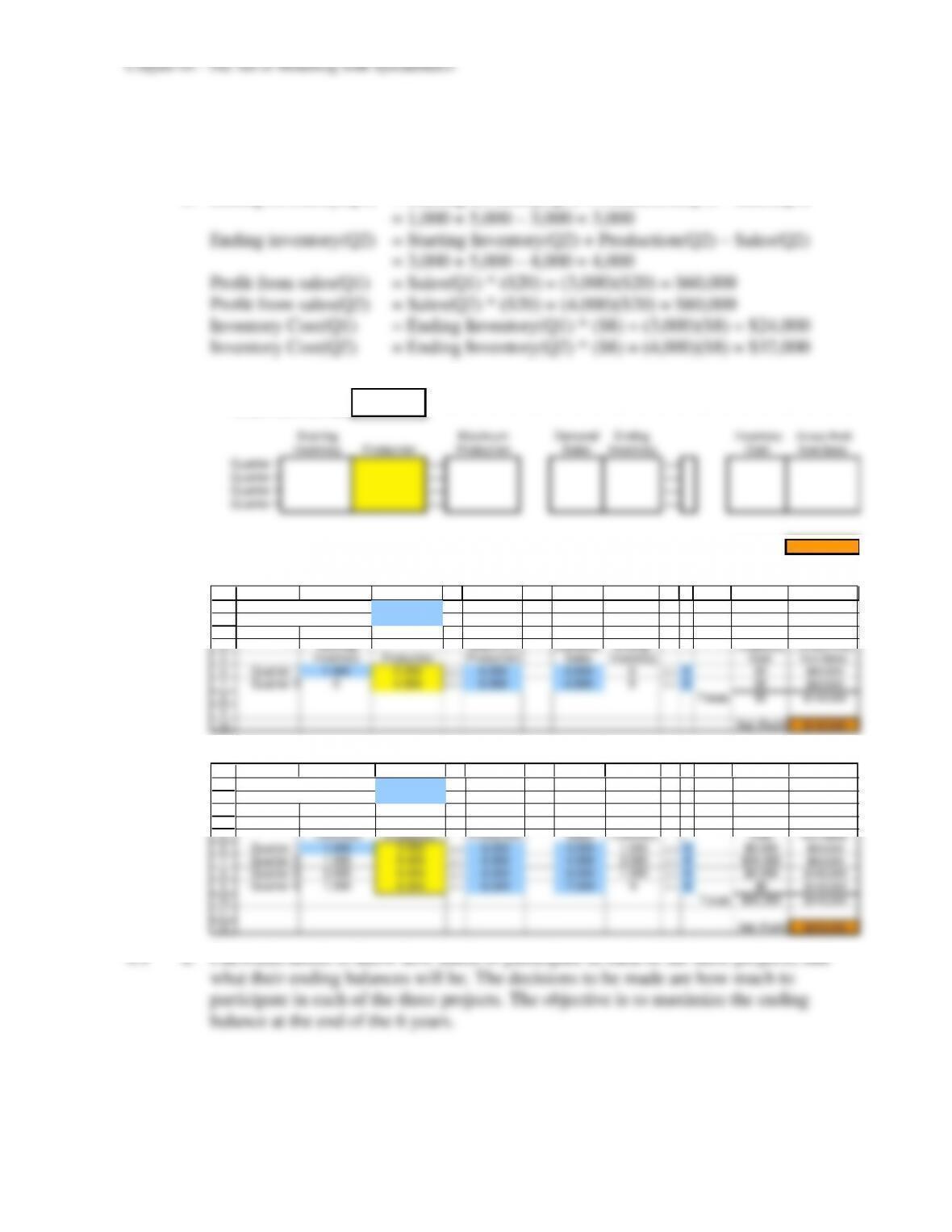
4.3 a. Top management will need to know how much to produce in each quarter. Thus, the
decisions are the production levels in quarters 1, 2, 3, and 4. The objective is to
maximize the net profit.
b. Ending inventory(Q1) = Starting Inventory(Q1) + Production(Q1) – Sales(Q1)
c.
Inventory Holding Cost
Gross Profit from Sales
Starting Maximum Demand/ Ending Inventory Gross Profit
Inventory Production Production Sales Inventory Cost from Sales
Quarter 1 <= >=
Quarter 2 <= >=
Quarter 3 <= >=
Quarter 4 <= >=
Net Profit
d.
1
2
3
4
5
6
7
8
9
10
A B C D E F G H I J K L M
Inventory Holding Cost $8
Gross Profit from Sales $20
Starting Maximum Demand/ Ending Inventory Gross Profit
Inventory Production Production Sales Inventory Cost from Sales
Quarter 1 1,000 2,000 <= 6,000 3,000 0 >= 0$0 $60,000
Quarter 2 0 4,000 <= 6,000 4,000 0 >= 0$0 $80,000
Totals $0 $140,000
Net Profit $140,000
e.
1
2
3
4
5
6
7
8
9
10
11
12
A B C D E F G H I J K L M
Inventory Holding Cost $8
Gross Profit from Sales $20
Starting Maximum Demand/ Ending Inventory Gross Profit
Inventory Production Production Sales Inventory Cost from Sales
Quarter 1 1,000 3,000 <= 6,000 3,000 1,000 >= 0 $8,000 $60,000
Quarter 2 1,000 6,000 <= 6,000 4,000 3,000 >= 0 $24,000 $80,000
Quarter 3 3,000 6,000 <= 6,000 8,000 1,000 >= 0 $8,000 $160,000
Quarter 4 1,000 6,000 <= 6,000 7,000 0 >= 0$0 $140,000
Totals $40,000 $440,000
Net Profit $400,000
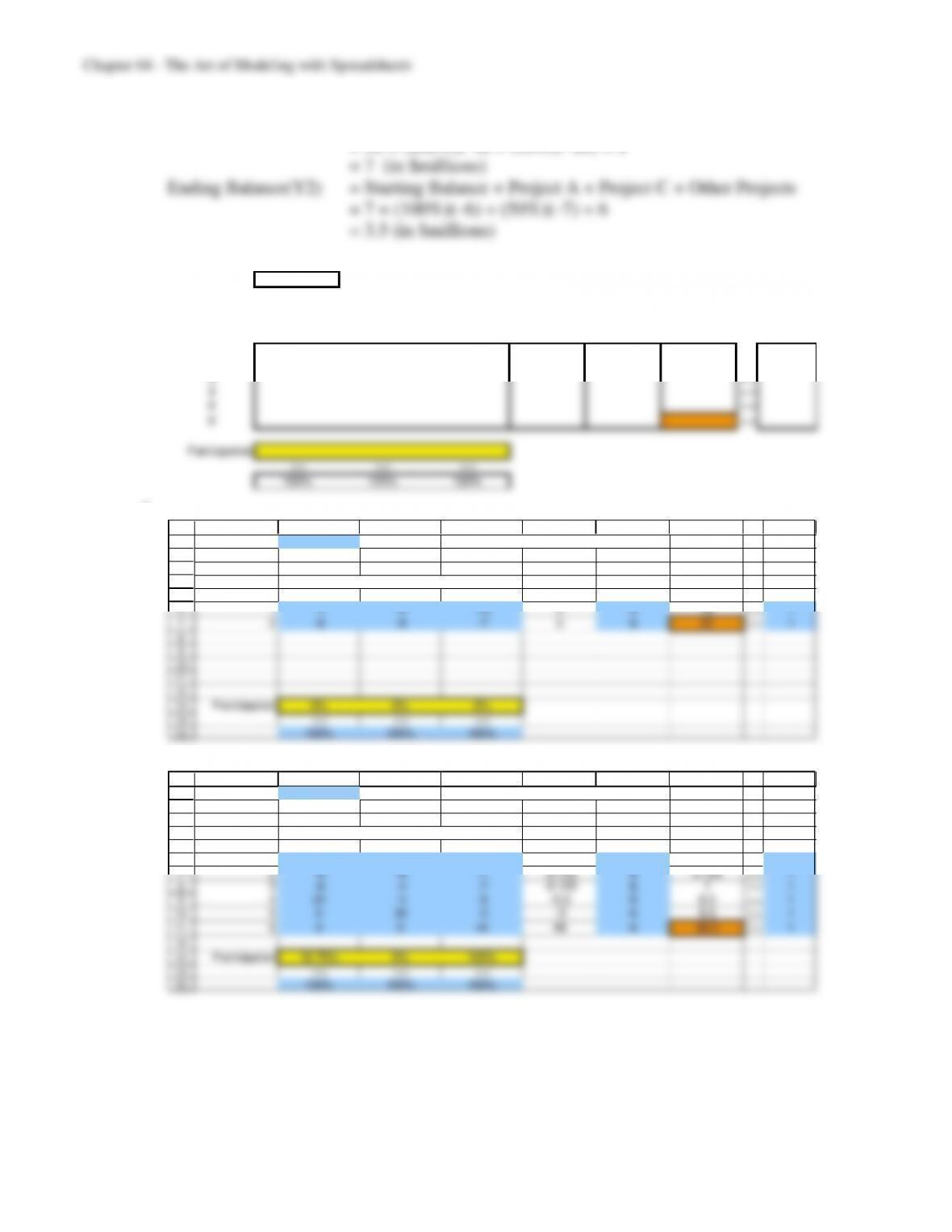
4.4 a. Fairwinds needs to know how much to participate in each of the three projects, and
what their ending balances will be. The decisions to be made are how much to
participate in each of the three projects. The objective is to maximize the ending
balance at the end of the 6 years.
4-4
b. Ending Balance(Y1) = Starting Balance + Project A + Project C + Other Projects
= 10 + (100%)(–4) + (50%)(–10) + 6
c.
Starting Cash
Total
Cash Flow (at full participation, $million) Cash Flow Other Ending Minimum
Year Project A Project B Project C From ABC Projects Balance Balance
1>=
2>=
3>=
4>=
5>=
6>=
Participation
<= <= <=
100% 100% 100%
d.
1
2
3
4
5
6
7
8
9
10
11
12
13
14
15
A B C D E F G H I
Starting Cash 10 all cash numbers are in $millions
Total
Cash Flow (at full participation, $million) Cash Flow Other Ending Minimum
Year Project A Project B Project C From ABC Projects Balance Balance
1-4 -8 -10 0 6 16 >= 1
2-6 -8 -7 0 6 22 >= 1
Participation 0% 0% 0%
<= <= <=
100% 100% 100%
e.
1
2
3
4
5
6
7
8
9
10
11
12
13
14
15
A B C D E F G H I
Starting Cash 10 all cash numbers are in $millions
Total
Cash Flow (at full participation, $million) Cash Flow Other Ending Minimum
Year Project A Project B Project C From ABC Projects Balance Balance
1-4 -8 -10 -10.75 6 5.25 >= 1
2-6 -8 -7 -8.125 6 3.125 >= 1
3-6 -4 -7 -8.125 6 1 >= 1
424 -4 -5 -0.5 6 6.5 >= 1
5 0 30 -3 -3 6 9.5 >= 1
6 0 0 44 44 6 59.5 >= 1
Participation 18.75% 0% 100%
<= <= <=
100% 100% 100%
4.5 Upon facing problems about juice logistics, Welch’s formulated the juice logistics model
(JLM), which is “an application of LP to a single-commodity network problem. The
decision variables deal with the cost of transfers between plants, the cost of recipes, and
carrying cost- all cost that are key to the common planning unit of tons” [p. 20]. The goal is
to find the optimal grape juice quantities shipped to customers and transferred between
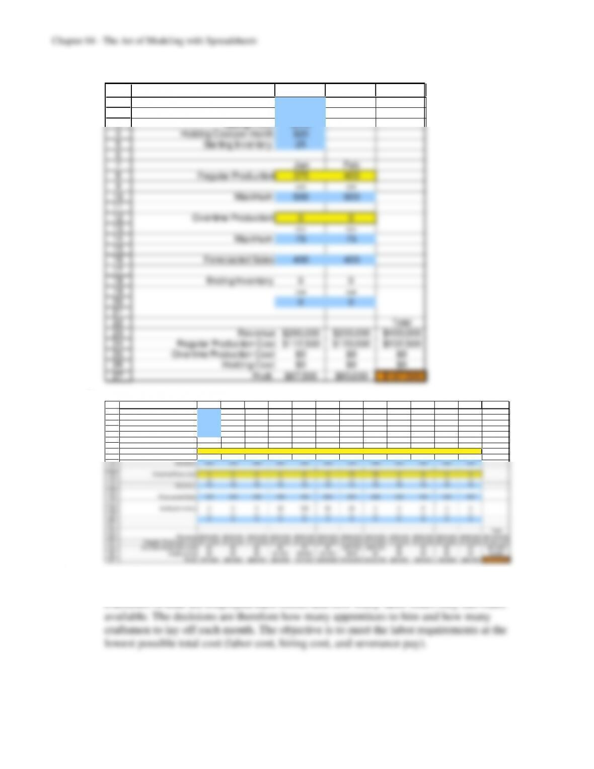
4.6 a. Decorum needs to know how many ceiling fans to produce each month with their
regular workforce and/or utilizing temporary workers. The decision variables are
therefore how many ceiling fans to produce with their regular work force and how
many to produce using temporary workers. The objective is to maximize their profit.
b. Regular Production Cost (Jan) = ($300)(450) = $135,000
Holding Cost (Jan) = ($20)(75) = $1,500
c.
Unit Production Cost (regular)
Unit Production Cost (OT)
Selling Price
Holding Cost per month
Starting Inventory
Jan Feb Mar Apr May Jun Jul Aug Sep Oct Nov Dec
Regular Production
<= <= <= <= <= <= <= <= <= <= <= <=
Maximum
Overtime Production
<= <= <= <= <= <= <= <= <= <= <= <=
Maximum
Forecasted Sales
Ending Inventory
>= >= >= >= >= >= >= >= >= >= >= >=
0 0 0 0 0 0 0 0 0 0 0 0
4-6
d.
1
2
3
4
5
6
7
8
9
10
11
12
13
14
15
16
17
18
19
20
21
22
23
24
25
26
27
A B C D
Unit Production Cost (regular) $300
Unit Production Cost (OT) $350
Selling Price $500
Holding Cost per month $20
Starting Inventory 25
Jan Feb
Regular Production 375 400
<= <=
Maximum 500 500
Overtime Production 0 0
<= <=
Maximum 75 75
Forecasted Sales 400 400
Ending Inventory 0 0
>= >=
0 0
Total
Revenue $200,000 $200,000 $400,000
Regular Production Cost $112,500 $120,000 $232,500
Overtime Production Cost $0 $0 $0
Holding Cost $0 $0 $0
Profit $87,500 $80,000 $167,500
e.
1
2
3
4
5
6
7
8
9
10
11
12
13
14
15
16
17
18
19
20
21
22
23
24
25
26
27
A B C D E F G H I J K L M N
Unit Production Cost (regular) $300
Unit Production Cost (OT) $350
Selling Price $500
Holding Cost per month $20
Starting Inventory 25
Jan Feb Mar Apr May Jun Jul Aug Sep Oct Nov Dec
Regular Production 375 400 400 450 500 500 500 500 400 400 400 400
<= <= <= <= <= <= <= <= <= <= <= <=
Maximum 500 500 500 500 500 500 500 500 500 500 500 500
Overtime Production 0 0 0 0 0 0 75 75 0 0 0 0
<= <= <= <= <= <= <= <= <= <= <= <=
Maximum 75 75 75 75 75 75 75 75 75 75 75 75
Forecasted Sales 400 400 400 400 400 600 600 600 400 400 400 400
Ending Inventory 0 0 0 50 150 50 25 00000
>= >= >= >= >= >= >= >= >= >= >= >=
000000000000
Total
Revenue $200,000 $200,000 $200,000 $200,000 $200,000 $300,000 $300,000 $300,000 $200,000 $200,000 $200,000 $200,000 $2,700,000
Regular Production Cost $112,500 $120,000 $120,000 $135,000 $150,000 $150,000 $150,000 $150,000 $120,000 $120,000 $120,000 $120,000 $1,567,500
Overtime Production Cost $0 $0 $0 $0 $0 $0 $26,250 $26,250 $0 $0 $0 $0 $52,500
Holding Cost $0 $0 $0 $1,000 $3,000 $1,000 $500 $0 $0 $0 $0 $0 $5,500
Profit $87,500 $80,000 $80,000 $64,000 $47,000 $149,000 $123,250 $123,750 $80,000 $80,000 $80,000 $80,000 $1,074,500
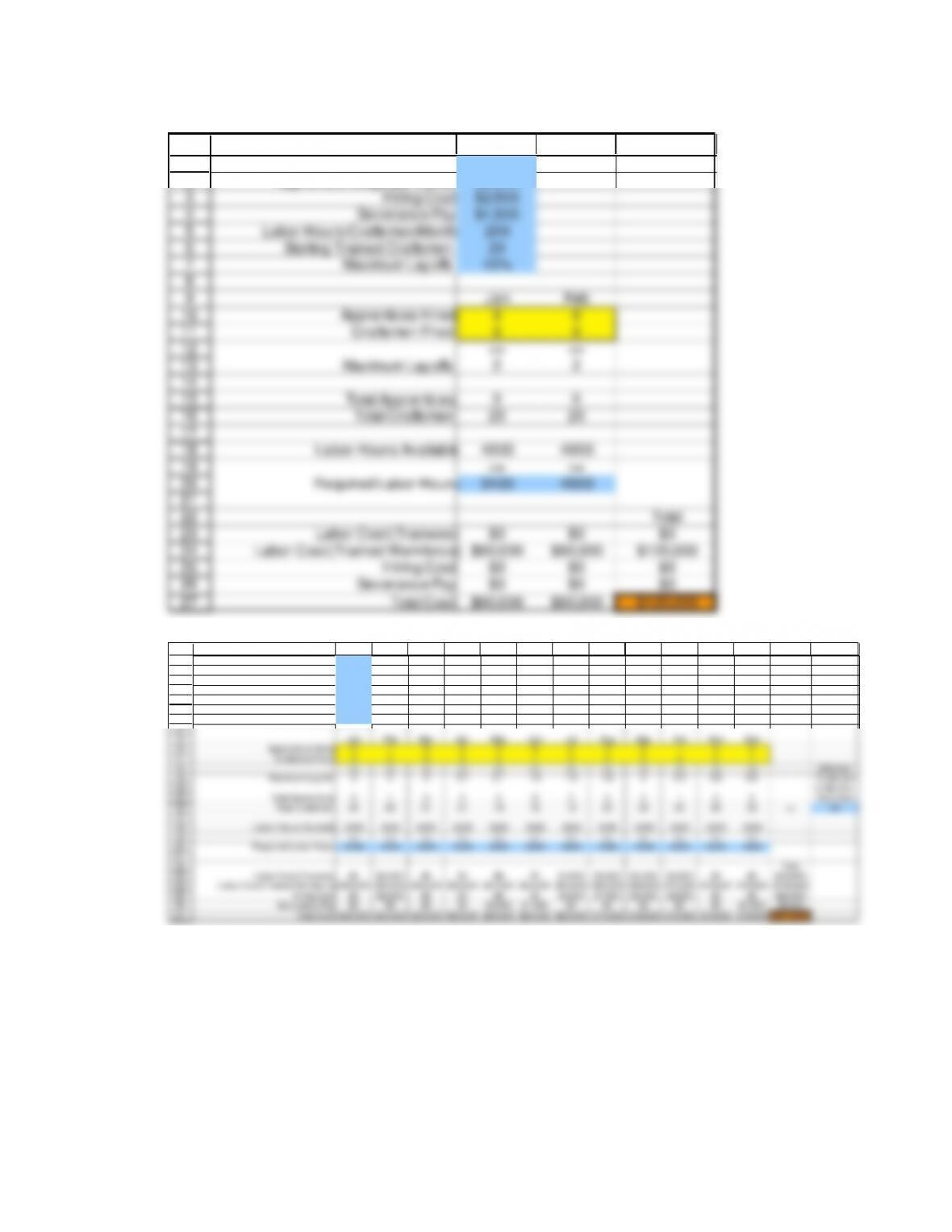
4.7 a. Allen Furniture needs to know how many apprentices to hire and how many craftsmen
to lay off each month. They will need to keep track of how many apprentices and
craftsmen in total are employed each month and how many labor hours they can make
4-7
b. In January there will be 20 craftsmen and 1 apprentice. The 20 craftsmen can make (20
craftsmen)(200 hours/craftsman) = 4000 labor-hours available. In February there will
be 21 craftsmen and no apprentices. The 21 craftsmen can make (21 craftsmen)(200
c.
Craftsman Wage per month
Apprentice Wage per month
Hiring Cost
Severance Pay
Labor Hours/Craftsman/Month
Starting Trained Craftsmen
Maximum Layoffs
Jan Feb Mar Apr May Jun Jul Aug Sep Oct Nov Dec
Apprentices Hired
Craftsmen Fired
<= <= <= <= <= <= <= <= <= <= <= <= Minimum
Maximum Layoffs 0 0 0 0 0 0 0 0 0 0 0 0 Craftsmen
to Start the
Total Apprentices Next Year
Total Craftsmen >=
Labor Hours Available
>= >= >= >= >= >= >= >= >= >= >= >=
Required Labor Hours
Total
Labor Cost (Trainees)
Labor Cost (Trained Workforce)
Hiring Cost
Severance Pay
Total Cost
Chapter 04 – The Art of Modeling with Spreadsheets
4-8
d.
1
2
3
4
5
6
7
8
9
10
11
12
13
14
15
16
17
18
19
20
21
22
23
24
25
26
27
A B C D
Craftsman Wage per month $3,000
Apprentice Wage per month $2,000
Hiring Cost $2,500
Severance Pay $1,500
Labor Hours/Craftsman/Month 200
Starting Trained Craftsmen 20
Maximum Layoffs 10%
Jan Feb
Apprentices Hired 0 0
Craftsmen Fired 0 0
<= <=
Maximum Layoffs 2 2
Total Apprentices 0 0
Total Craftsmen 20 20
Labor Hours Available 4000 4000
>= >=
Required Labor Hours 3400 4000
Total
Labor Cost (Trainees) $0 $0 $0
Labor Cost (Trained Workforce) $60,000 $60,000 $120,000
Hiring Cost $0 $0 $0
Severance Pay $0 $0 $0
Total Cost $60,000 $60,000 $120,000
e.
1
2
3
4
5
6
7
8
9
10
11
12
13
14
15
16
17
18
19
20
21
22
23
24
25
26
27
A B C D E F G H I J K L M N O
Craftsman Wage per month $3,000
Apprentice Wage per month $2,000
Hiring Cost $2,500
Severance Pay $1,500
Labor Hours/Craftsman/Month 200
Starting Trained Craftsmen 20
Maximum Layoffs 10%
Jan Feb Mar Apr May Jun Jul Aug Sep Oct Nov Dec
Apprentices Hired 0 1 0 0 0 0 2 3 2 1 0 0
Craftsmen Fired 0 0 0 0 2 1 0 0 0 0 0 1
<= <= <= <= <= <= <= <= <= <= <= <= Minimum
Maximum Layoffs 2 2 2 2.1 2.1 1.9 1.8 1.8 2 2.3 2.5 2.6 Craftsmen
to Start the
Total Apprentices 0 1 0 0 0 0 2 3 2 1 0 0 Next Year
Total Craftsmen 20 20 21 21 19 18 18 20 23 25 26 25 >= 25
Labor Hours Available 4000 4000 4200 4200 3800 3600 3600 4000 4600 5000 5200 5000
>= >= >= >= >= >= >= >= >= >= >= >=
Required Labor Hours 3400 4000 4200 4200 3000 2800 3000 4000 4500 5000 5200 4800
Total
Labor Cost (Trainees) $0 $2,000 $0 $0 $0 $0 $4,000 $6,000 $4,000 $2,000 $0 $0 $18,000
Labor Cost (Trained Workforce)$60,000 $60,000 $63,000 $63,000 $57,000 $54,000 $54,000 $60,000 $69,000 $75,000 $78,000 $75,000 $768,000
Hiring Cost $0 $2,500 $0 $0 $0 $0 $5,000 $7,500 $5,000 $2,500 $0 $0 $22,500
Severance Pay $0 $0 $0 $0 $3,000 $1,500 $0 $0 $0 $0 $0 $1,500 $6,000
Total Cost $60,000 $64,500 $63,000 $63,000 $60,000 $55,500 $63,000 $73,500 $78,000 $79,500 $78,000 $76,500 $814,500
4.8 a. Web Mercantile needs to know each month how many square feet to lease and for how
long. The decisions therefore are for each month how many square feet to lease for one
month, for two months, for three months, etc. The objective is to minimize the overall
leasing cost.
4-9
b. Total Cost = (30,000 square feet)($190 per square foot)
c.
Month Covered by Lease? Total Space
Month of Lease: 1 1 1 1 1 2 2 2 2 3 3 3 4 4 5 Leased Required
Length of Lease: 1 2 3 4 5 1 2 3 4 1 2 3 1 2 1 (sq. ft.) (sq. ft.)
Month 1 >=
Month 2 >=
Month 3 >=
Month 4 >=
Month 5 >=
Cost of Lease
(per sq. ft.)
Total Cost
Lease (sq. ft.)
d.
1
2
3
4
5
6
7
8
9
10
A B C D E F G
Month Covered by Lease? Total Space
Month of Lease: 1 1 2 Leased Required
Length of Lease: 1 2 1 (sq. ft.) (sq. ft.)
Month 1 1 1 30,000 >= 30,000
Month 2 1 1 20,000 >= 20,000
Cost of Lease $65 $100 $65
(per sq. ft.)
Total Cost
Lease (sq. ft.) 10,000 20,000 0 $2,650,000
e.
1
2
3
4
5
6
7
8
9
10
11
12
13
A B C D E F G H I J K L M N O P Q R S
Month Covered by Lease? Total Space
Month of Lease: 1 1 1 1 1 2 2 2 2 3 3 3 4 4 5 Leased Required
Length of Lease: 1 2 3 4 5 1 2 3 4 1 2 3 1 2 1 (sq. ft.) (sq. ft.)
Month 1 1 1 1 1 1 30,000 >= 30,000
Month 2 1 1 1 1 1 1 1 1 30,000 >= 20,000
Month 3 1 1 1 1 1 1 1 1 1 40,000 >= 40,000
Month 4 1 1 1 1 1 1 1 1 30,000 >= 10,000
Month 5 1 1 1 1 1 50,000 >= 50,000
Cost of Lease $65 $100 $135 $160 $190 $65 $100 $135 $160 $65 $100 $135 $65 $100 $65
(per sq. ft.)
Total Cost
Lease (sq. ft.) 0 0 0 0 30,000 0 0 0 0 10,000 0 0 0 0 20,000 $7,650,000
4.9 a. Larry needs to know how many employees should work each possible shift. Therefore,
the decision variables are the number of employees that work each shift. The objective
is to minimize the total cost of the employees.
b. Working 8am-noon: 3 FT morning + 3 PT = 6
4-10
c.
Full Time Full Time Full Time Part Time Part Time Part Time Part Time
8am-4pm noon-8pm 4pm-midnight 8am–noon noon–4pm 4pm-8pm 8pm-midnight
Cost per Shift
Total Total
Shift Covers Time of Day? (1=yes, 0=no) Working Needed
8am-noon >=
noon-4pm >=
4pm-8pm >=
8pm-midnight >=
Workers per Shift
Total Times Total Total
Time of Day Full Time Part Time Cost
8am-noon >=
noon-4pm >=
4pm-8pm >=
8pm-midnight >=
d.
1
2
3
4
5
6
7
8
9
10
11
12
13
14
15
16
17
18
19
A B C D E F G H I J K
Full Time Full Time Full Time Part Time Part Time Part Time Part Time
8am-4pm noon–8pm 4pm-midnight 8am-noon noon-4pm 4pm-8pm 8pm-midnight
Cost per Shift $112 $112 $112 $48 $48 $48 $48
Total Total
Shift Covers Time of Day? (1=yes, 0=no) Working Needed
8am-noon 1 1 6 >= 6
noon–4pm 1 1 1 8 >= 8
4pm-8pm 1 1 1 12 >= 12
8pm-midnight 1 1 6 >= 6
Workers per Shift 4 2 6 2 2 4 0
2
Total Times Total Total
Time of Day Full Time Part Time Cost
8am-noon 4 >= 4 $1,728
noon–4pm 6 >= 4
4pm-8pm 8 >= 8
8pm-midnight 6 >= 0
4.10 a. Al will need to know how much to invest in each possible investment each year. Thus,
the decisions are how much to invest in investment A in year 1, 2, 3, and 4; how much
b. Ending Cash (Y1) = $60,000 (Starting Balance) – $20,000 (A in Y1) = $40,000
4-12
4.11 In the poor formulation, the data are not separated from the formula—they are buried
inside the equations in column C. In contrast, the spreadsheet in Figure 4.6 separates all of
the data in their own cells, and then the formulas for hours used and total profit refer to
these data cells.
The poor formulation does not show the entire model on the spreadsheet. There is no
indication of the constraints on the spreadsheet (they are only displayed in the Solver
4.12 Cell F16 has –0.47 for LT Interest, rather than –LTRate*LTLoan.
4.13 Cell G21 for the 2021 ST Interest uses LTRate instead of STRate.
Case
4.1 a. PFS needs to know how many units of each of the four bonds to purchase, how much to
invest in the money market, and their ending balance in the money market fund each
4-13
b. Payment received from Bond 1 (2012) = (10 thousand units) ($1,000 face value) +
(10,000 units) ($1,000 face value) (0.04 coupon rate) = $10.4 million
Payment received from Bond 1 (2013) = $0
Balance in money market fund (2012) = $20 million (starting balance)
+ $10.4 million (payment from Bond 1)
+ $0.2 million (payment from Bond 2)
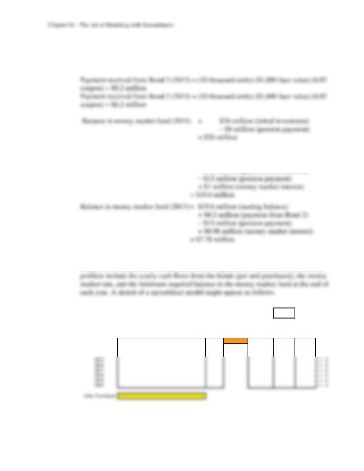
c. PFS will need to track the flow of cash from bond investments, the initial investment,
the required pension payments, interest from the money market, and the money market
balance. The decisions are the number of units to purchase of each bond. Data for the
Money Market Rate
Minimum Required Balance
Required Money Money
Bond Initial Pension Market Market
Bond 1 Bond 2 Bond 3 Bond 4 Flow Investment Flow Interest Balance
2011 >= 0
2012 >= 0
2013 >= 0
2014 >= 0
2015 >= 0
2016 >= 0
2017 >= 0
2018 >= 0
2019 >= 0
2020 >= 0
Units Purchased
Bond Cash Flows (per unit)
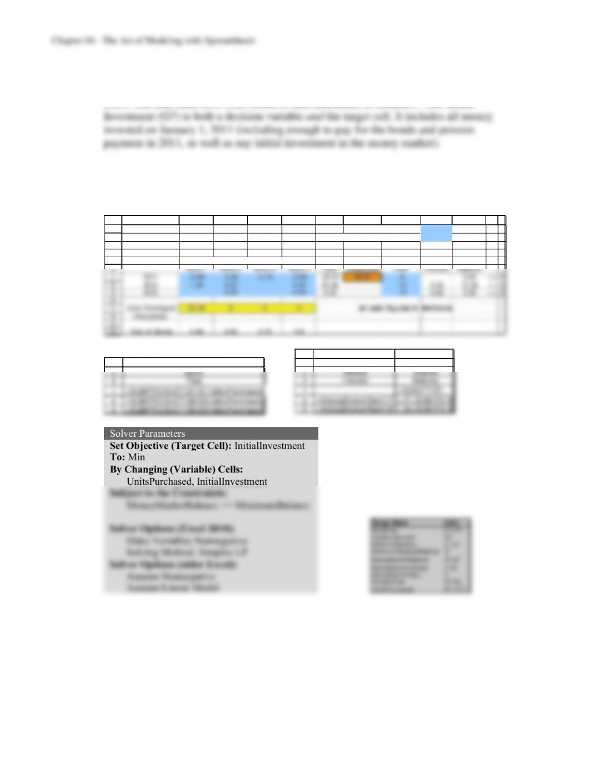
d. The bond cash flows (per unit) are calculated in B7:E9. For example, one unit of Bond
1 costs $0.98 in 2011, and returns the face value ($1) plus the coupon rate ($0.04) in
2008. The total cash flow from bonds is then calculated in column F. The Initial
If just years 2011 through 2013 are considered, then 23.44 thousand units of Bond 1
should be purchased at a cost of $22.97 million, along with an initial $8 million
investment in the money market fund on January 1, 2011.
1
2
3
4
5
6
7
8
9
10
11
12
13
A B C D E F G H I J K L
Money Market Rate 5%
Minimum Required Balance 0
Required Money Money
Bond Initial Pension Market Market
Bond 1 Bond 2 Bond 3 Bond 4 Flow Investment Flow Interest Balance
2011 –0.98 -0.92 -0.75 -0.80 -22.97 30.97 -8 0.00 >= 0
2012 1.04 0.02 0.03 24.38 –12 0.00 12.38 >= 0
2013 0.02 0.03 0.00 -13 0.62 0.00 >= 0
Units Purchased 23.44 0 0 0 all cash figures in $millions
(thousands)
Bond Cash Flows (per unit)
5
6
7
8
9
F
Bond
Flow
=SUMPRODUCT(B7:E7,UnitsPurchased)
=SUMPRODUCT(B8:E8,UnitsPurchased)
=SUMPRODUCT(B9:E9,UnitsPurchased)
4
5
6
7
8
9
I J
Money Money
Market Market
Interest Balance
=SUM(F7:I7)
=MoneyMarketRate*J7 =J7+SUM(F8:I8)
=MoneyMarketRate*J8 =J8+SUM(F9:I9)
Range Name Cells
BondFlow F7:F9
InitialInvestment G7
MinimumBalance L7:L9
MinimumRequiredBalance I2
MoneyMarketBalance J7:J9
MoneyMarketInterest I7:I9
MoneyMarketRate I1
PensionFlow H7:H9
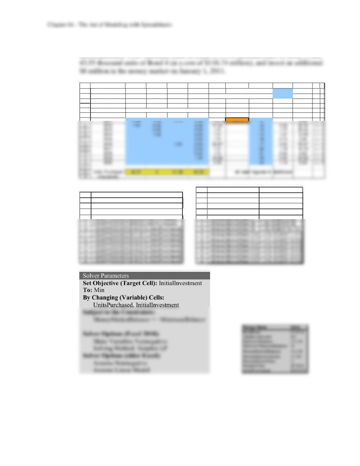
e. Expanded to consider all years through 2020, the spreadsheet is as shown below. PFS
should purchase 44.27 thousand units of Bond 1, 51.36 thousand units of Bond 3, and
1
2
3
4
5
6
7
8
9
10
11
12
13
14
15
16
17
18
A B C D E F G H I J K L
Money Market Rate 5%
Minimum Required Balance 0
Required Money Money
Bond Initial Pension Market Market
Bond 1 Bond 2 Bond 3 Bond 4 Flow Investment Flow Interest Balance
2011 -0.98 -0.92 -0.75 -0.80 –116.74 124.74 -8 0.00 >= 0
2012 1.04 0.02 0.03 47.34 –12 0.00 35.34 >= 0
2013 0.02 0.03 1.31 -13 1.77 25.42 >= 0
2014 1.02 0.03 1.31 -14 1.27 13.99 >= 0
2015 0.03 1.31 -16 0.70 0.00 >= 0
2016 1.00 0.03 52.67 –17 0.00 35.67 >= 0
2017 0.03 1.31 -20 1.78 18.76 >= 0
2018 0.03 1.31 -21 0.94 0.00 >= 0
2019 1.03 44.86 -22 0.00 22.86 >= 0
2020 0.00 –24 1.14 0.00 >= 0
Units Purchased 44.27 0 51.36 43.55 all cash figures in $millions
Bond Cash Flows (per unit)
5
6
7
8
9
10
11
12
13
14
15
16
F
Bond
Flow
=SUMPRODUCT(B7:E7,UnitsPurchased)
=SUMPRODUCT(B8:E8,UnitsPurchased)
=SUMPRODUCT(B9:E9,UnitsPurchased)
=SUMPRODUCT(B10:E10,UnitsPurchased)
=SUMPRODUCT(B11:E11,UnitsPurchased)
=SUMPRODUCT(B12:E12,UnitsPurchased)
=SUMPRODUCT(B13:E13,UnitsPurchased)
=SUMPRODUCT(B14:E14,UnitsPurchased)
=SUMPRODUCT(B15:E15,UnitsPurchased)
=SUMPRODUCT(B16:E16,UnitsPurchased)
4
5
6
7
8
9
10
11
12
13
14
15
16
I J
Money Money
Market Market
Interest Balance
=SUM(F7:I 7)
=MoneyMarketRate*J7 =J7+SUM(F8:I8)
=MoneyMarketRate*J8 =J8+SUM(F9:I9)
=MoneyMarketRate*J9 =J9+SUM(F10:I10)
=MoneyMarketRate*J10 =J10+SUM(F11:I11)
=MoneyMarketRate*J11 =J11+SUM(F12:I12)
=MoneyMarketRate*J12 =J12+SUM(F13:I13)
=MoneyMarketRate*J13 =J13+SUM(F14:I14)
=MoneyMarketRate*J14 =J14+SUM(F15:I15)
=MoneyMarketRate*J15 =J15+SUM(F16:I16)
Range Name Cells
BondFlow F7:F16
InitialInvestment G7
MinimumBalance L7:L16
MinimumRequiredBalance I2
MoneyMarketBalance J7:J16
MoneyMarketInterest I7:I16
MoneyMarketRate I1
PensionFlow H7:H16
UnitsPurchased B18:E18