CD2s-1
CD Supplement to Chapter 2 More About the Graphical Method for
Linear Programming
Problems
2s.1 Optimal Solution = (A, B) = (x1, x2) = (0.667, 0.667). P = $3333.33.
CD2s-2
2s.3 Optimal Solution: (x1, x2) = (2, 3) and Z = 12.
b)
CD2s-3
b)
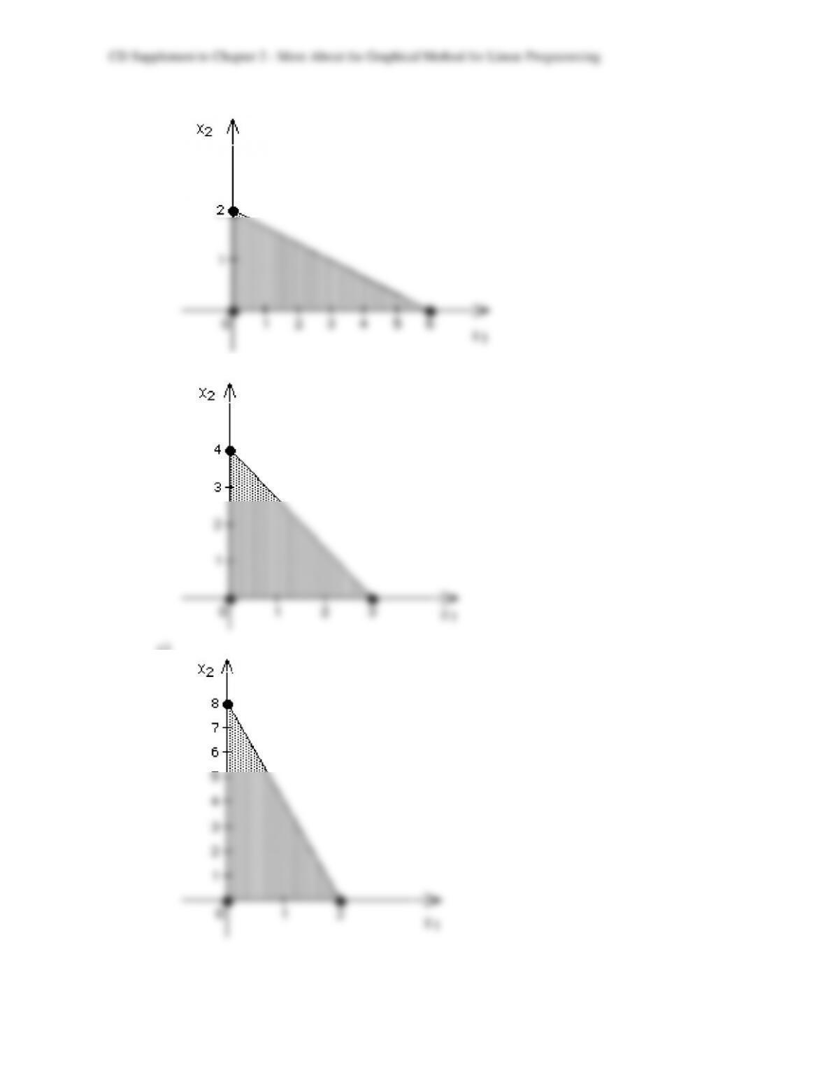
2s.6 a) If x2 = 0 then x1 = 6. If x1 = 0 then x2 = –4.
b)
c) slope = 0.667
CD2s-4
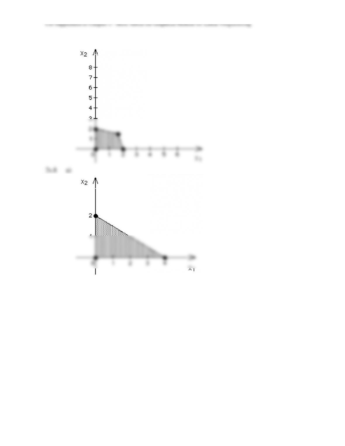
2s.7 a)
b)
c)
CD2s-5
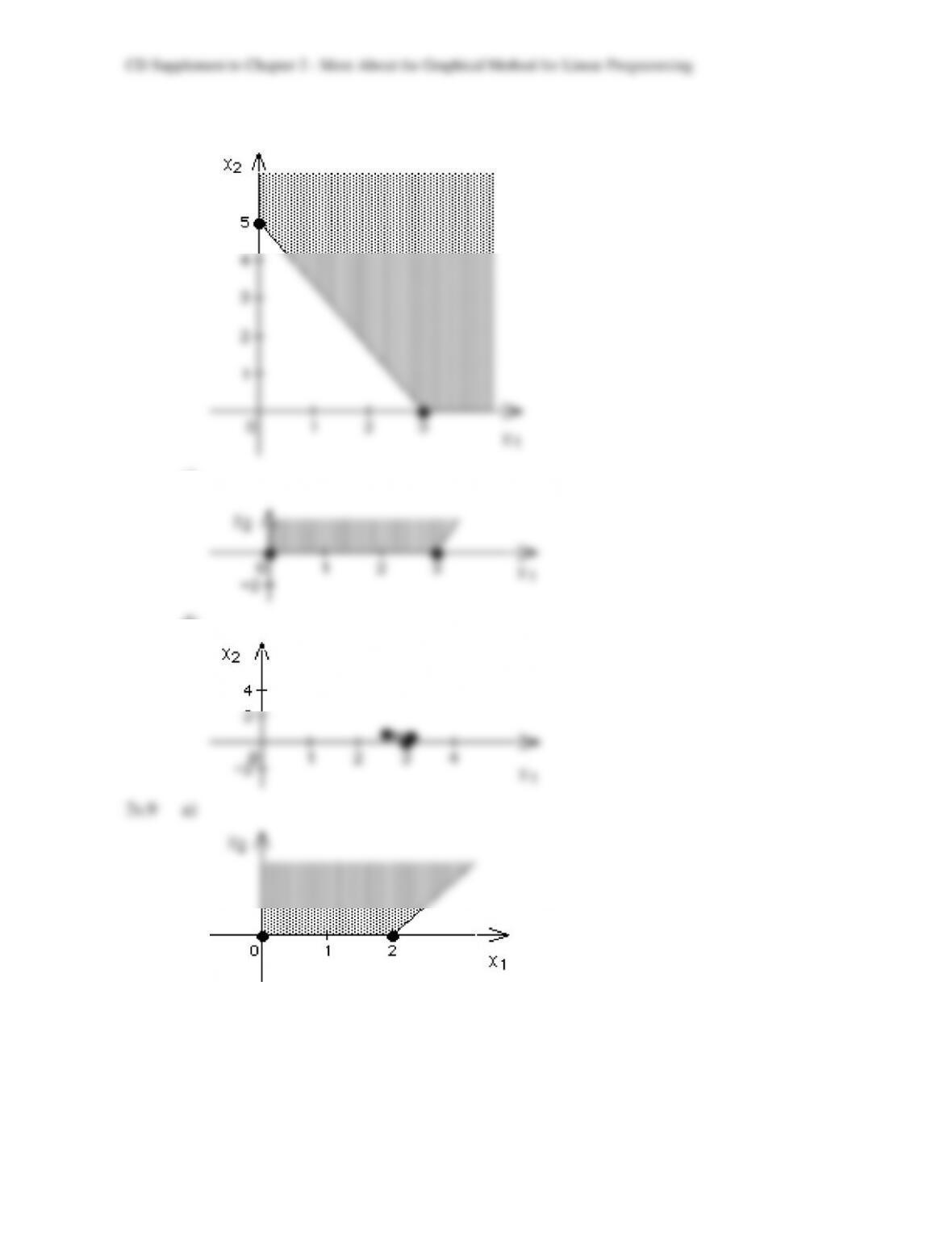
d)
CD2s-6
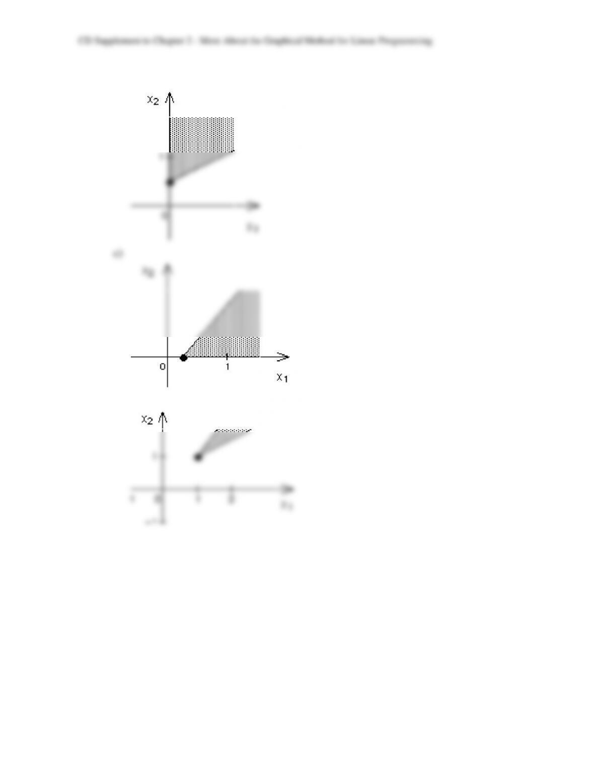
b)
c)
d)
CD2s-7
b)
d)
CD2s-8
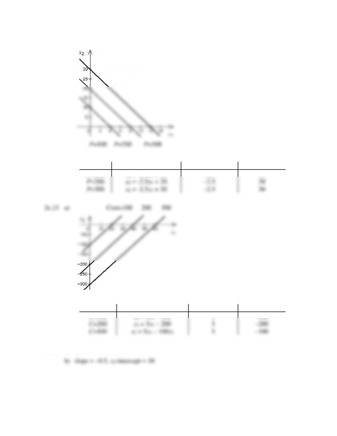
2s.11 a)
b)
slope-intercept form
slope
x2 intercept
P=6
x2 = –0.667x1 + 2
–0.667
2
P=12
x2 = –0.667x1 + 4
–0.667
4
P=18
x2 = –0.667x1 + 6
–0.667
6
CD Supplement to Chapter 2 – More About the Graphical Method for Linear Programming
CD2s-9
2s.12 a)
b)
slope-intercept form
slope
x2 intercept
P=100
x2 = -2.5x1 + 10
–2.5
10
P=200
x2 = -2.5x1 + 20
–2.5
20
P=300
x2 = -2.5x1 + 30
–2.5
30
b)
slope-intercept form
slope
x2 intercept
C=300
x2 = 5x1 – 300
5
–300
C=200
x2 = 5x1 – 200
5
–200
C=100
x2 = 5x1 – 100x2
5
–100
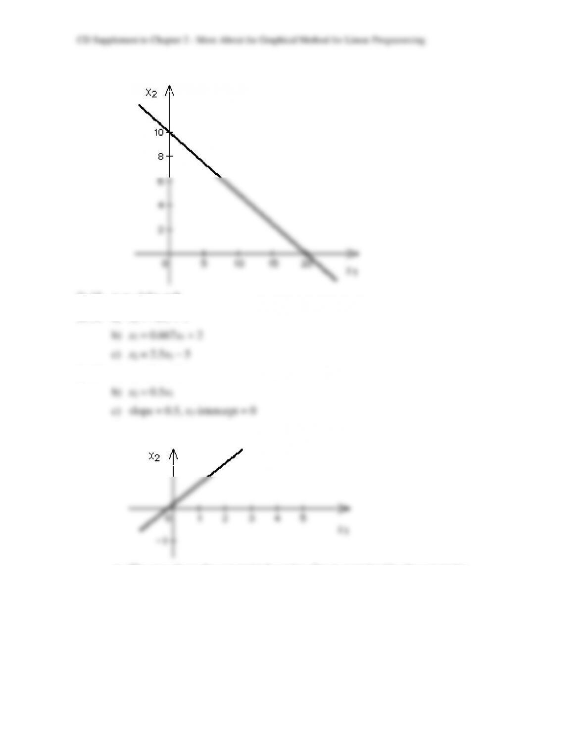
2s.14 a) x2 = –0.5x1 + 10
CD2s-10
c)
2s.15 x2 = –1.6x1 + 8
2s.16 a) x2 = –2x1 + 4
2s.17 a) x1 – 2x2 = 0
d)
e) The area above the constraint boundary line is permitted by the constraint.
CD2s-11
CD2s-12
CD2s-13
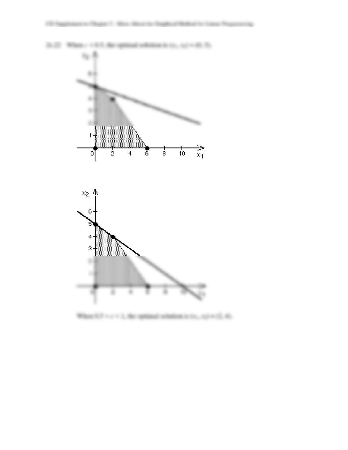
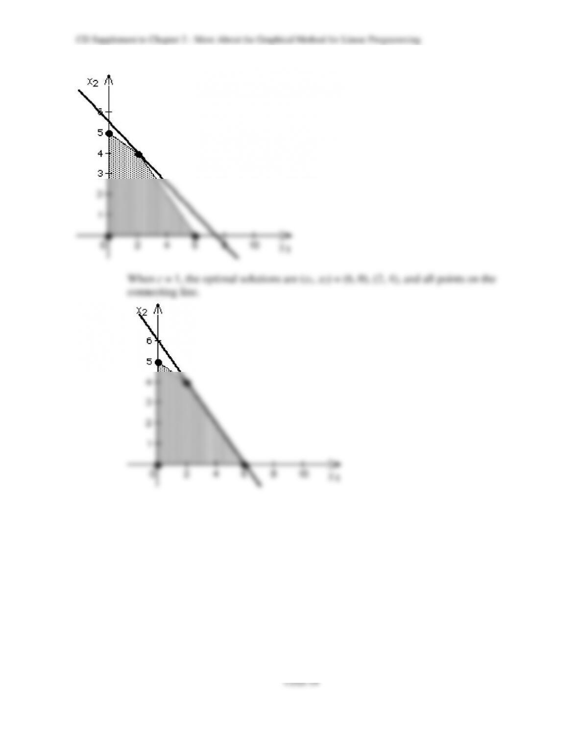
When c = 0.5, the optimal solutions are (x1, x2) = (0, 5), (2, 4), and all points on the
connecting line.
CD2s-14
CD2s-15
CD2s-16
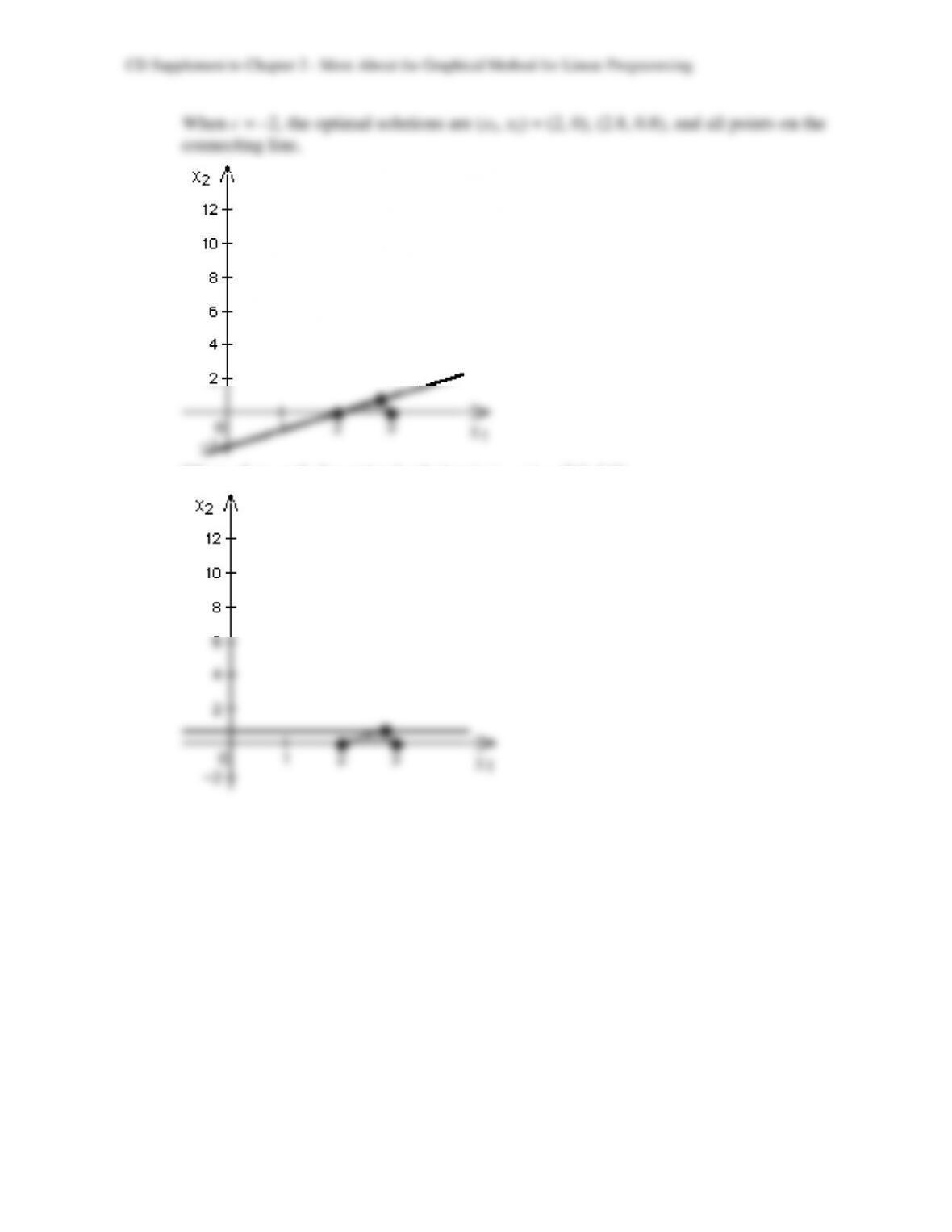
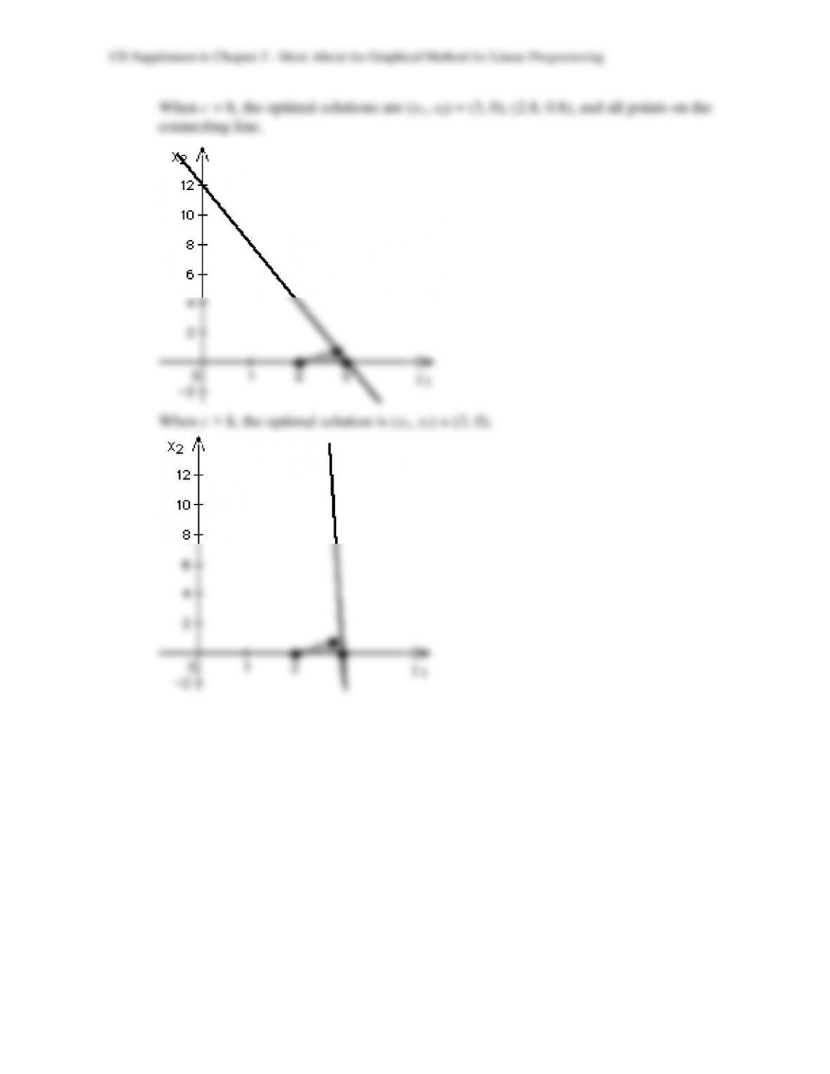
When –2 < c < 8, the optimal solution is (x1, x2) = (2.8, 0.8).
CD2s-17
CD2s-18
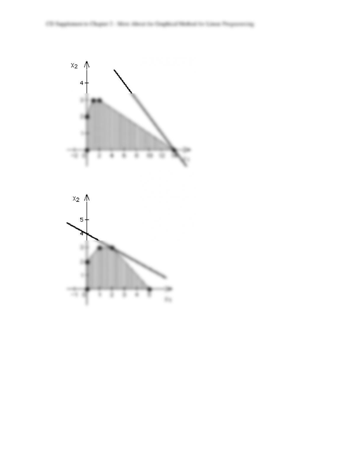
2s.24 When k < 0.5 (for example, k = 0.25 is graphed below), the optimal solution is (x1, x2) =
([2k+3]/k, 0). Thus, (2, 30) is not optimal for these values of k.
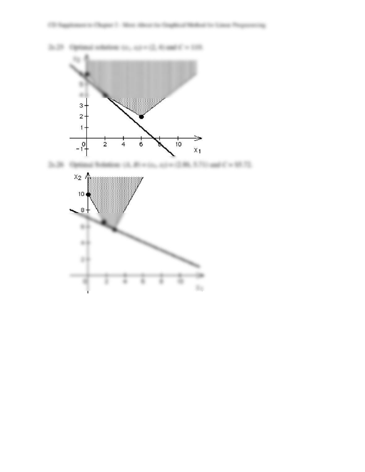
When k ≥ 0.5 (for example, k = 1 is graphed below), the optimal solution is (x1, x2) = (2,
3).
CD2s-19