2-1
Chapter 2 Linear Programming: Basic Concepts
Review Questions
2.1-1 1) Should the company launch the two new products?
2) What should be the product mix for the two new products?
2.1-2 The group was asked to analyze product mix.
2.1-3 Which combination of production rates for the two new products would maximize the total
profit from both of them.
2-2
2.3-3 A decision variable is an algebraic variable that represents a decision regarding the level of
a particular activity. The objective function is the part of a linear programming model that
expresses what needs to be either maximized or minimized, depending on the objective for
the problem. A nonnegativity constraint is a constraint that express the restriction that a
particular decision variable must be greater than or equal to zero. All constraints that are
not nonnegativity constraints are referred to as functional constraints.
2.3-4 A feasible solution is one that satisfies all the constraints of the problem. The best feasible
solution is called the optimal solution.
2-3
Problems
2.1 Swift & Company solved a series of LP problems to identify an optimal production
schedule. The first in this series is the scheduling model, which generates a shift-level
schedule for a 28-day horizon. The objective is to minimize the difference of the total cost
and the revenue. The total cost includes the operating costs and the penalties for shortage
2.2 a)
1
2
3
4
5
6
7
8
9
10
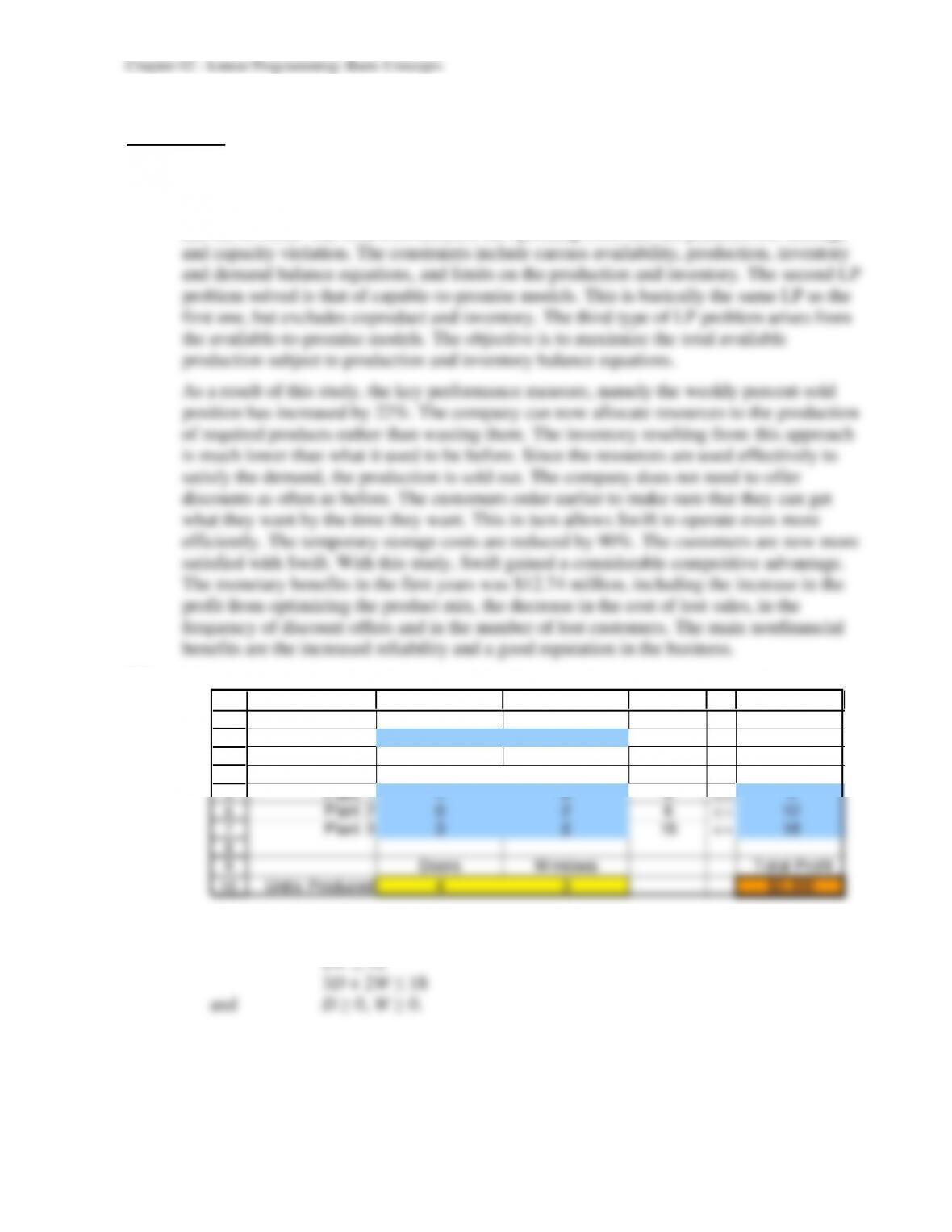
A B C D E F
Doors Windows
Unit Profit $600 $300
Hours Hours
Used Available
Plant 1 1 0 4 <= 4
Plant 2 0 2 6 <= 12
Plant 3 3 2 18 <= 18
Doors Windows Total Profit
Units Produced 4 3 $3,300
Hours Used Per Unit Produced
b) Maximize P = $600D + $300W,
subject to D ≤ 4
2W ≤ 12
2-4
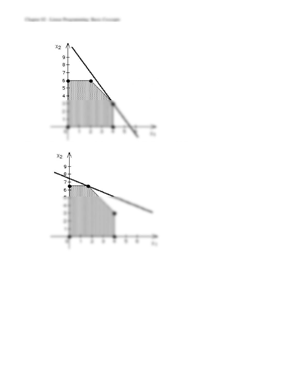
c) Optimal Solution = (D, W) = (x1, x2) = (4, 3). P = $3300.
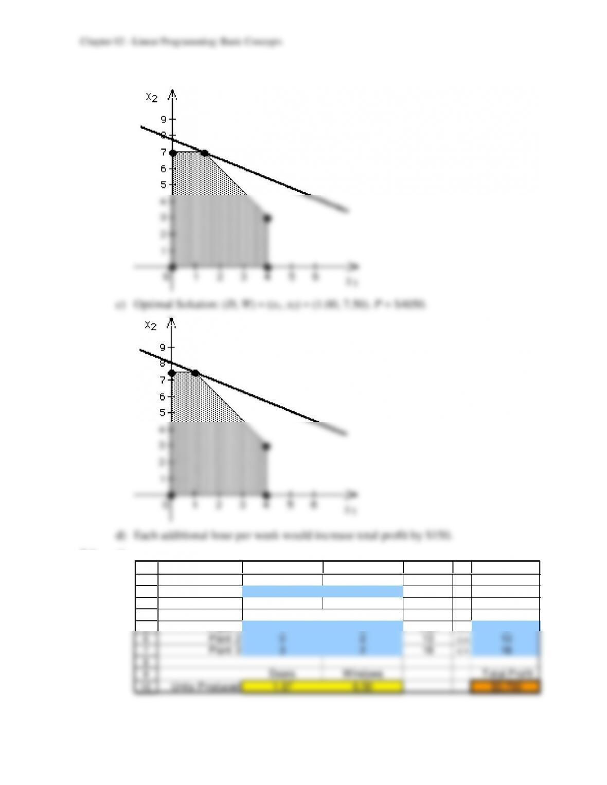
2.3 a) Optimal Solution: (D, W) = (x1, x2) = (1.67, 6.50). P = $3750.
2-5
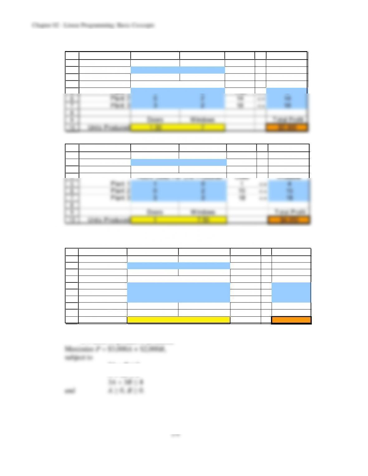
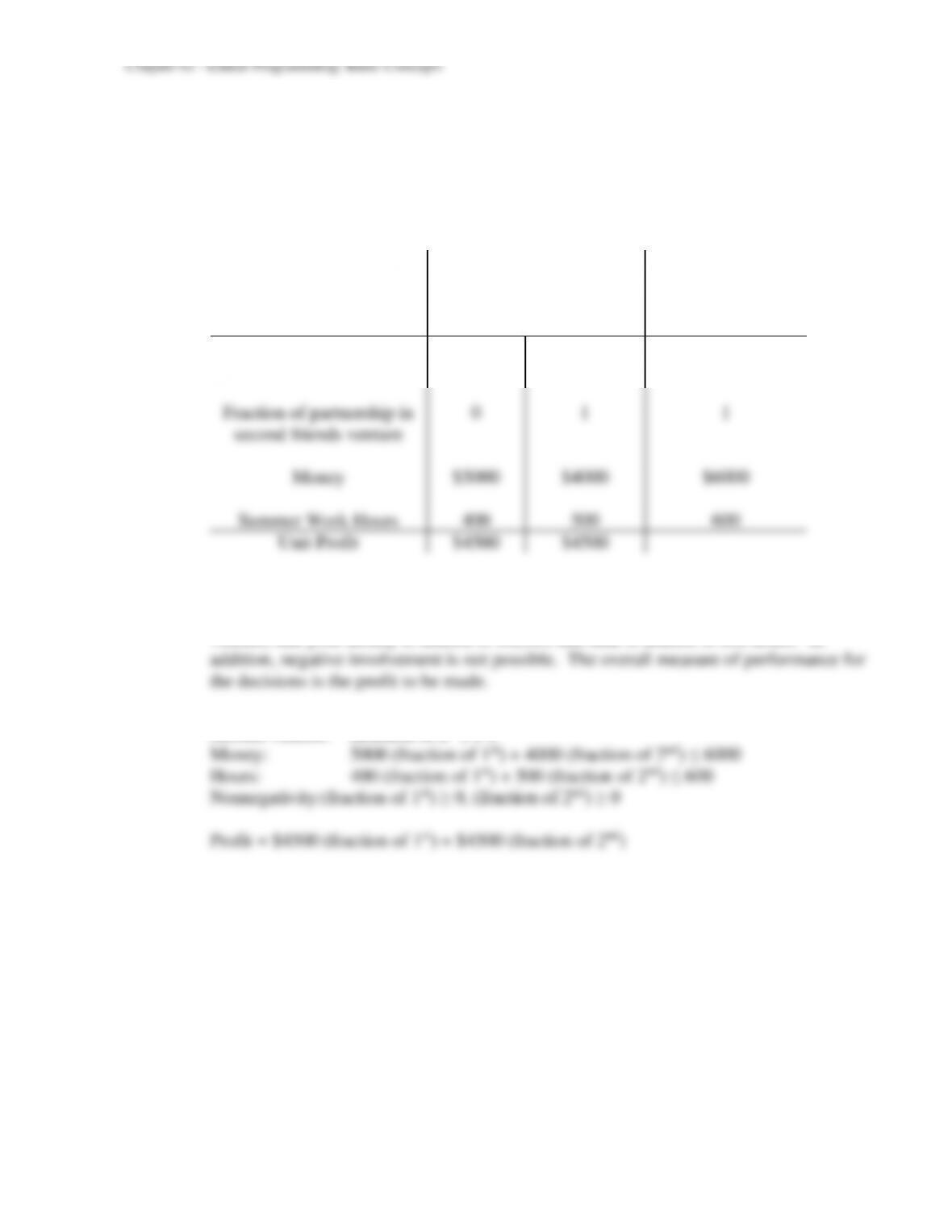
b) Optimal Solution: (D, W) = (x1, x2) = (1.33, 7.00). P = $3900.
2.4 a)
1
2
3
4
5
6
7
8
9
10
A B C D E F
Doors Windows
Unit Profit $300 $500
Hours Hours
Used Available
Plant 1 1 0 1.67 <= 4
Plant 2 0 2 13 <= 13
Plant 3 3 2 18 <= 18
Doors Windows Total Profit
Units Produced 1.67 6.50 $3,750
Hours Used Per Unit Produced
2-7
2.6 a) As in the Wyndor Glass Co. problem, we want to find the optimal levels of two
activities that compete for limited resources.
Let x1 be the fraction purchased of the partnership in the first friends venture.
Let x2 be the fraction purchased of the partnership in the second friends venture.
The following table gives the data for the problem:
Resource Usage
per Unit of Activity
Amount of
Resource
1
2
Resource
Available
Fraction of partnership in
first friends venture
1
0
1
Fraction of partnership in
second friends venture
0
1
1
Money
$5000
$4000
$6000
Summer Work Hours
400
500
600
Unit Profit
$4500
$4500
b) The decisions to be made are how much, if any, to participate in each venture. The
constraints on the decisions are that you can’t become more than a full partner in either
venture, that your money is limited to $6,000, and time is limited to 600 hours. In
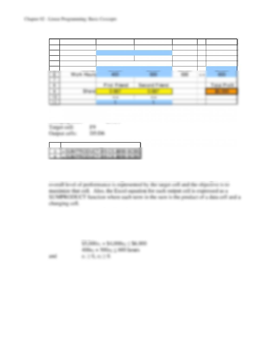
c) First venture: (fraction of 1st) ≤ 1
Second venture: (fraction of 2nd) ≤ 1
2-8
d)
1
2
3
4
5
6
7
8
9
10
11
A B C D E F
First Friend Second Friend
Unit Profit $4,500 $4,500
Resource Resource
Used Available
Money $5,000 $4,000 $6,000 <= $6,000
Work Hours 400 500 600 <= 600
First Friend Second Friend Total Profit
Share 0.667 0.667 $6,000
<= <=
Resource Usage
Data cells: B2:C2, B5:C6, F5:F6, and B11:C11
Changing cells: B9:C9
5
6
D
= SUMPRODUCT (B 5:C5, $B$9:$C$9)
= SUMPRODUCT (B 6:C6, $B$9:$C$9)
e) This is a linear programming model because the decisions are represented by changing
cells that can have any value that satisfy the constraints. Each constraint has an output
cell on the left, a mathematical sign in the middle, and a data cell on the right. The
f) Let x1 = share taken in first friend’s venture
x2 = share taken in second friend’s venture
Maximize P = $4,500x1 + $4,500x2,
subject to x1 ≤ 1
x2 ≤ 1
2-9
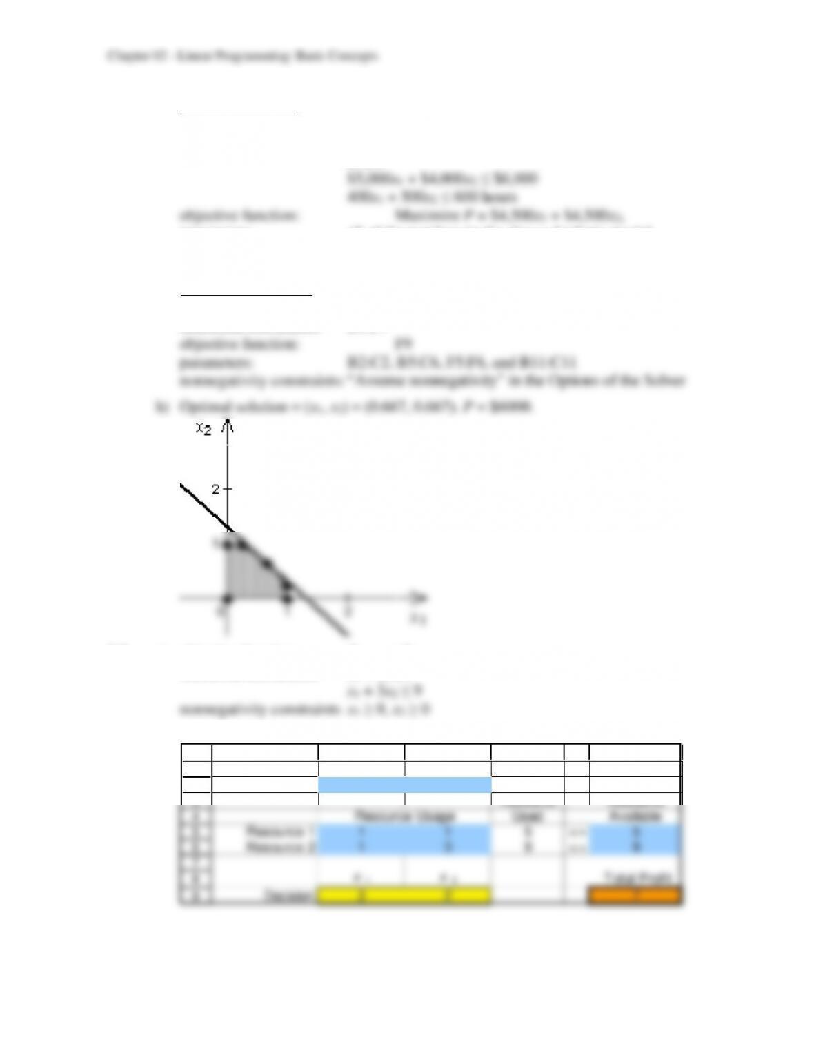
g) Algebraic Version
decision variables: x1, x2
functional constraints: x1 ≤ 1
x2 ≤ 1
parameters: all of the numbers in the above algebraic model
nonnegativity constraints: x1 ≥ 0, x2 ≥ 0
Spreadsheet Version
decision variables: B9:C9
functional constraints: D4:F7
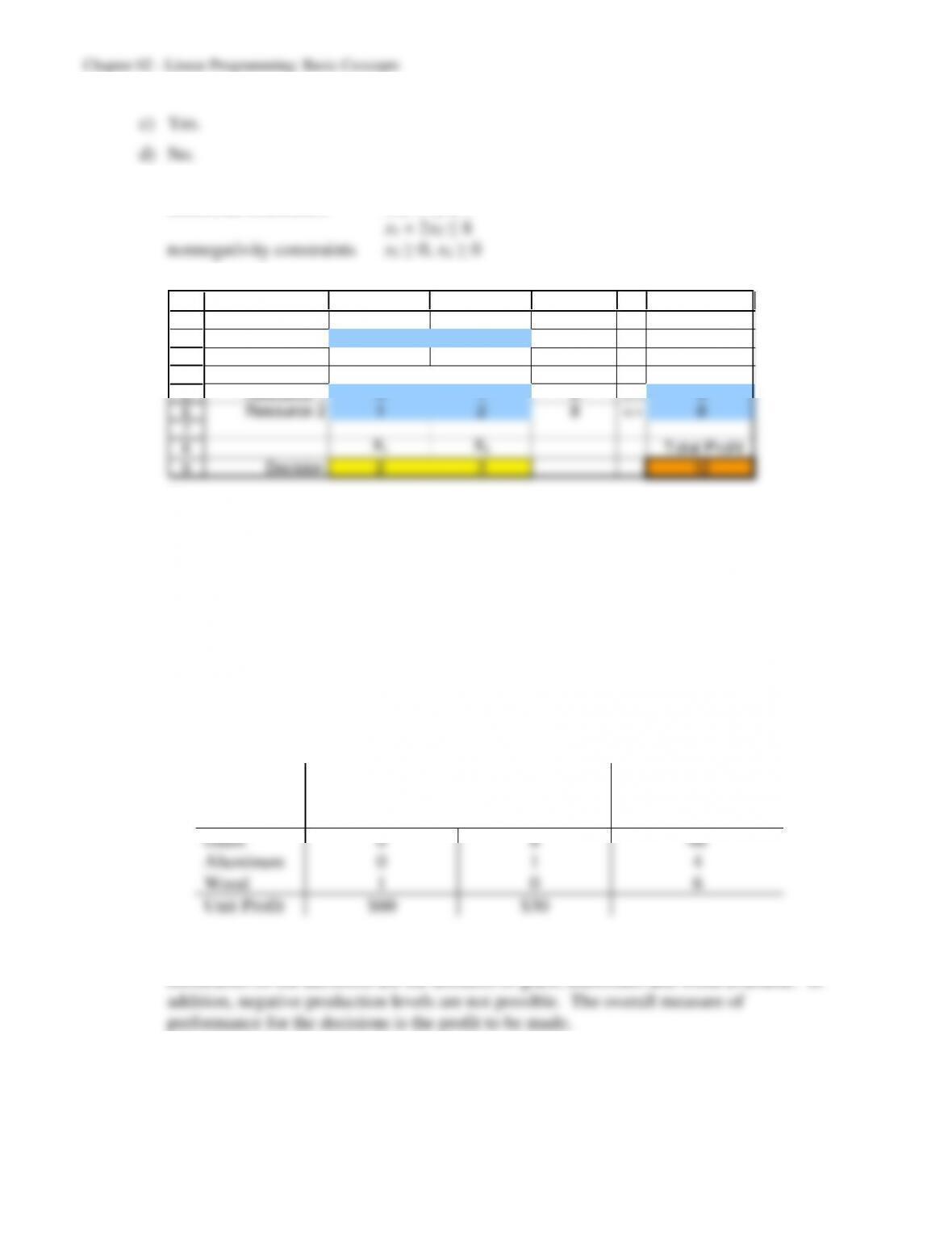
2.7 a) objective function Z = x1 + 2x2
functional constraints x1 + x2 ≤ 5
b & e)
1
2
3
4
5
6
7
8
9
A B C D E F
x1x2
Unit Profit 1 2
Resource Resource
Used Available
Resource 1 1 1 5 <= 5
Resource 2 1 3 9 <= 9
x1x2Total Profit
Decision 3 2 7
Resource Usage
2-10
2.8 a) objective function Z = 3x1 + 2x2
functional constraints 3x1 + x2 ≤ 9
b & f)
1
2
3
4
5
6
7
8
9
A B C D E F
X1X2
Unit Profit 3 2
Resource Resource
Used Available
Resource 1 3 1 9 <= 9
Resource 2 1 2 8 <= 8
X1X2Total Profit
Decision 2 3 12
Resource Usage
c) Yes.
d) Yes.
e) No.
2.9 a) As in the Wyndor Glass Co. problem, we want to find the optimal levels of two
activities that compete for limited resources. We want to find the optimal mix of the
two activities.
Let W be the number of wood-framed windows to produce.
Let A be the number of aluminum-framed windows to produce.
The following table gives the data for the problem:
Resource Usage per Unit of Activity
Amount of
Resource
Wood-framed
Aluminum-
framed
Resource Available
Glass
6
8
48
Aluminum
0
1
4
Wood
1
0
6
Unit Profit
$60
$30
b) The decisions to be made are how many windows of each type to produce. The
constraints on the decisions are the amounts of glass, aluminum and wood available. In
2-11
c) glass: 6 (#wood-framed) + 8 (# aluminum-framed) ≤ 48
Profit = $60 (#wood-framed) + $30 (# aluminum-framed)
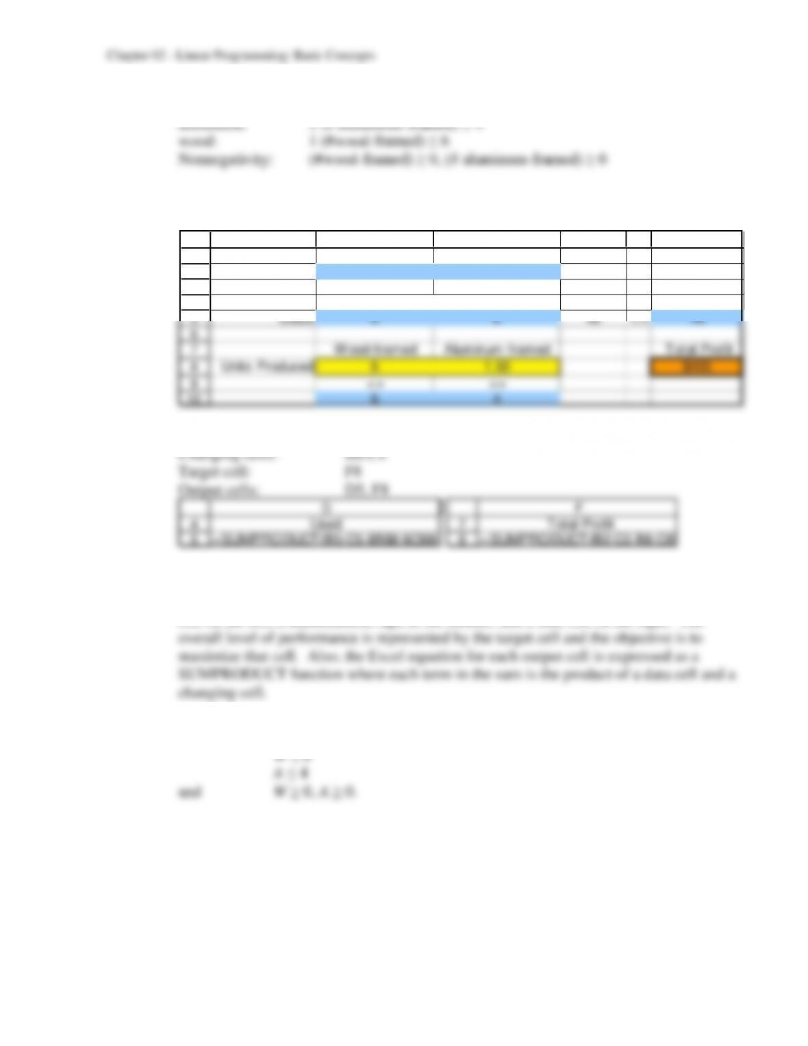
d)
1
2
3
4
5
6
7
8
9
10
A B C D E F
Wood-framed Aluminum–framed
Unit Profit $60 $30
Used Available
Glass 6 8 48 <= 48
Wood-framed Aluminum–framed Total Profit
Units Produced 6 1.50 $405
<= <=
6 4
Square-feet Used Per Unit Produced
Data cells: B2:C2, B5:C5, F5, B10:C10
e) This is a linear programming model because the decisions are represented by changing
cells that can have any value that satisfy the constraints. Each constraint has an output
cell on the left, a mathematical sign in the middle, and a data cell on the right. The
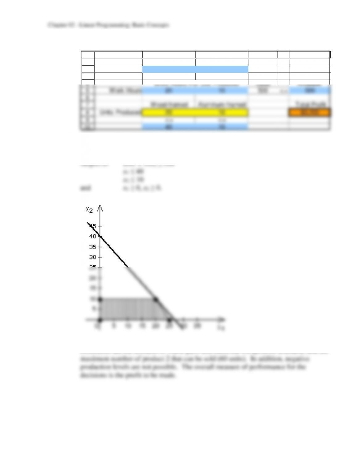
f) Maximize P = 60W + 30A
subject to 6W + 8A ≤ 48
2-12
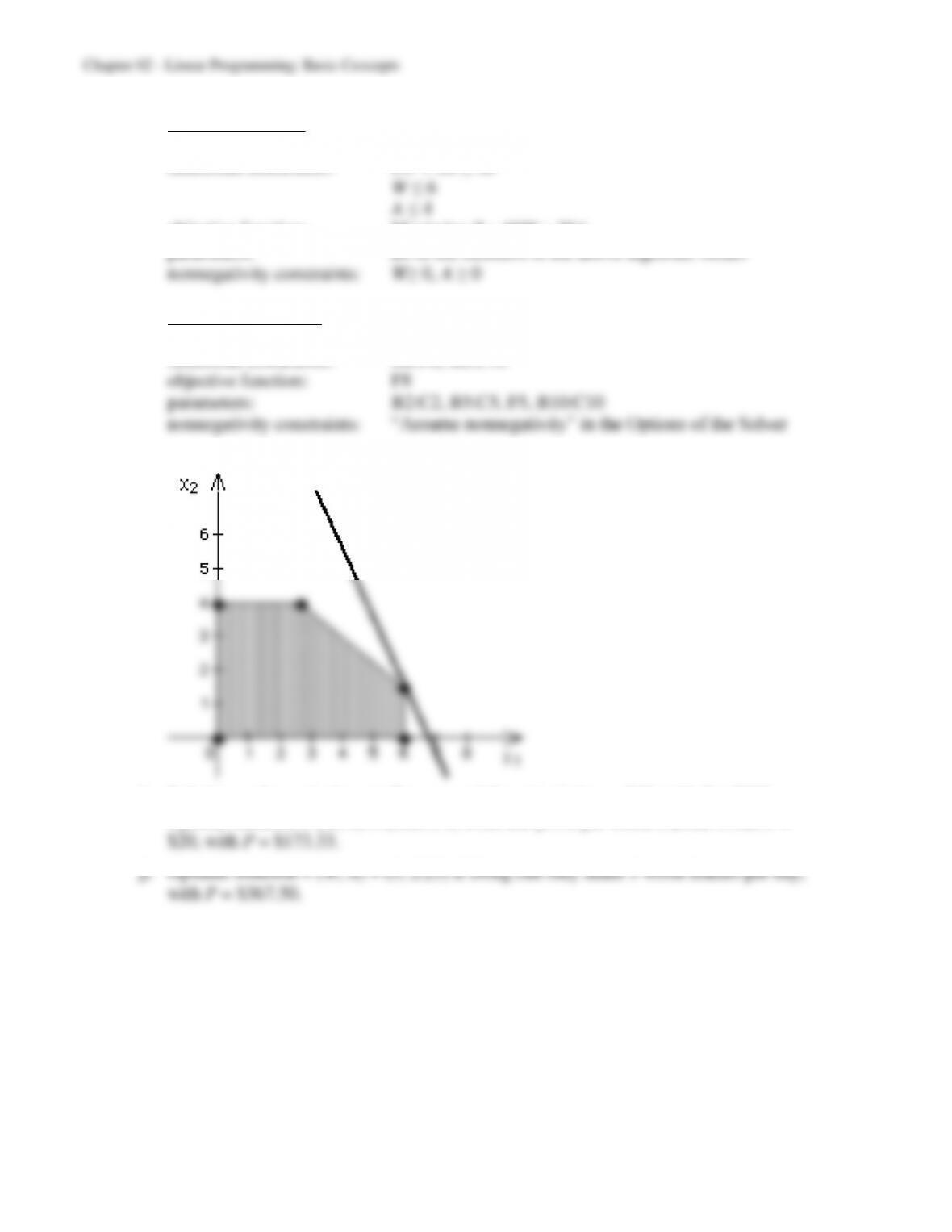
g) Algebraic Version
decision variables: W, A
functional constraints: 6W + 8A ≤ 48
objective function: Maximize P = 60W + 30A
parameters: all of the numbers in the above algebraic model
Spreadsheet Version
decision variables: B8:C8
functional constraints: D8:F8, B8:C10
h) Optimal Solution: (W, A) = (x1, x2) = (6, 1.5) and P = $405.
i) Solution unchanged when profit per wood-framed window = $40, with P = $285.
Optimal Solution = (W, A) = (2.667, 4) when the profit per wood-framed window =
2-13
2.10 a)
1
2
3
4
5
6
7
8
9
10
A B C D E F
27″ Sets 20″ Sets
Unit Profit $120 $80
Hours Hours
Used Available
Work Hours 20 10 500 <= 500
Wood-framed Aluminum–framed Total Profit
Units Produced 20 10 $3,200
<= <=
40 10
Work Hours Per Unit Produced
b) Let x1 = number of 27” TV sets to be produced per month
Let x2 = number of 20” TV sets to be produced per month
Maximize P = $120x1 + $80x2,
c) Optimal Solution: (x1, x2) = (20, 10) and P = $3200.
2.11 a) The decisions to be made are how many of each light fixture to produce. The
constraints are the amounts of frame parts and electrical components available, and the
2-14
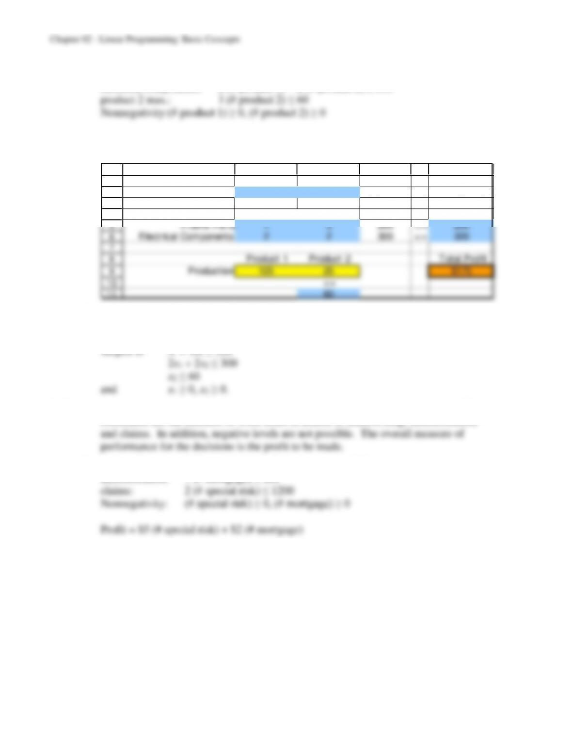
b) frame parts: 1 (# product 1) + 3 (# product 2) ≤ 200
electrical components: 2 (# product 1) + 2 (# product 2) ≤ 300
Profit = $1 (# product 1) + $2 (# product 2)
c)
1
2
3
4
5
6
7
8
9
10
11
A B C D E F
Product 1 Product 2
Unit Profit $1 $2
Resource Resource
Used Available
Frame Parts 1 3 200 <= 200
Electrical Components 2 2 300 <= 300
Product 1 Product 2 Total Profit
Production 125 25 $175
<=
Resource Usage
d) Let x1 = number of units of product 1 to produce
x2 = number of units of product 2 to produce
Maximize P = $1x1 + $2x2,
subject to x1 + 3x2 ≤ 200
2.12 a) The decisions to be made are what quotas to establish for the two product lines. The
constraints are the amounts of work hours available in underwriting, administration,
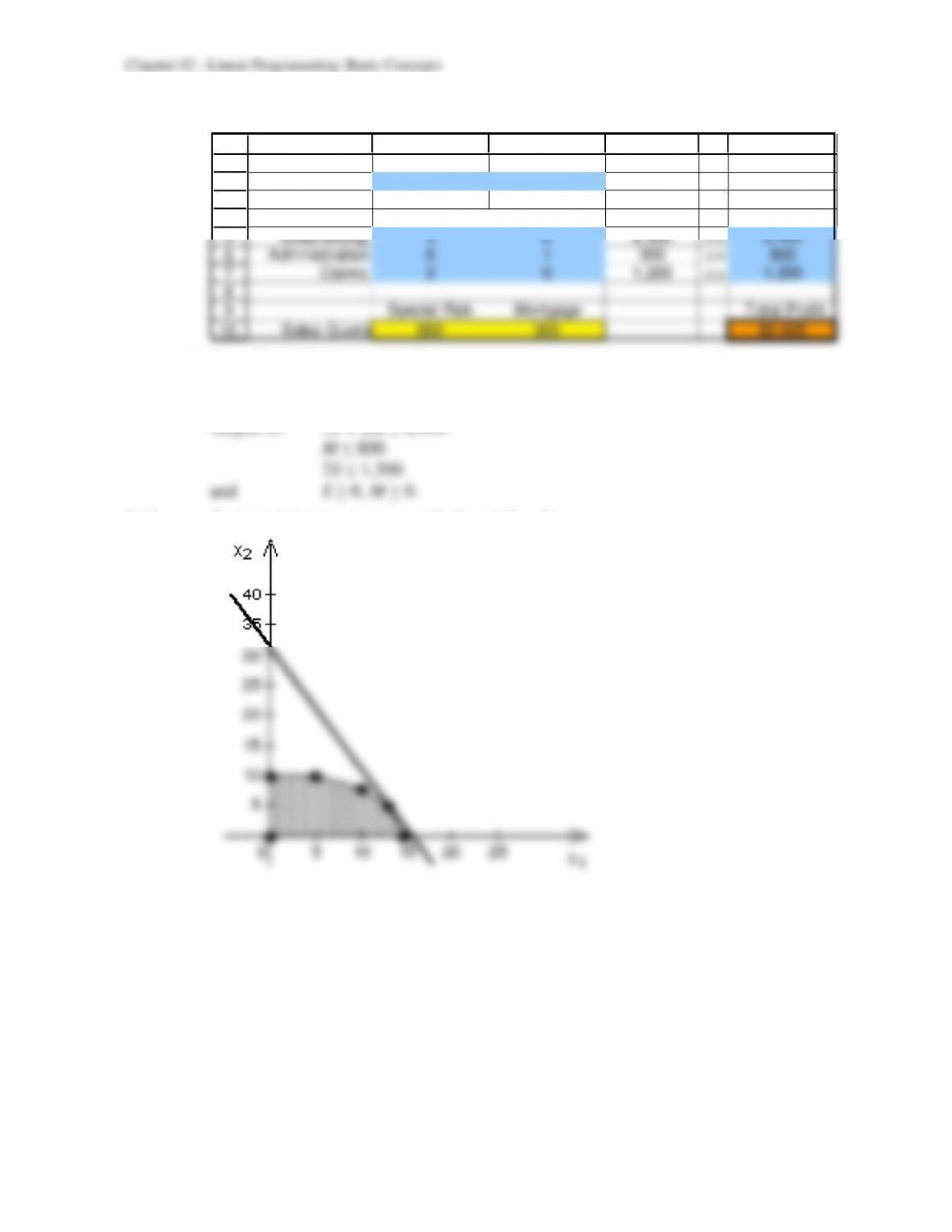
b) underwriting: 3 (# special risk) + 2 (# mortgage) ≤ 2400
administration: 1 (# mortgage) ≤ 800
2-15
c)
1
2
3
4
5
6
7
8
9
10
A B C D E F
Special Risk Mortgage
Unit Profit $5 $2
Work-Hours W ork–Hours
Used Available
Underwriting 3 2 2,400 <= 2,400
Administration 0 1 300 <= 800
Claims 2 0 1,200 <= 1,200
Special Risk Mortgage Total Profit
Sales Quota 600 300 $3,600
Work-Hours per Unit
d) Let S = units of special risk insurance
M = units of mortgages
Maximize P = $5S + $2M,
subject to 3S + 2M ≤ 2,400
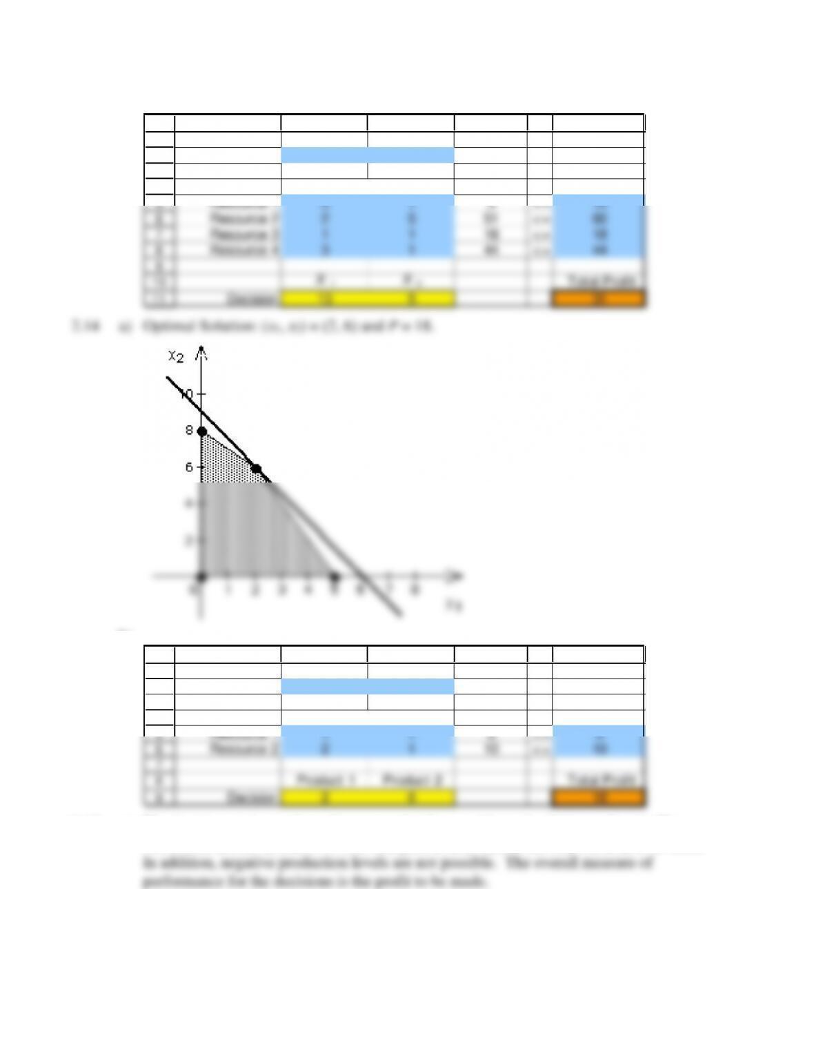
2.13 a) Optimal Solution: (x1, x2) = (13, 5) and P = 31.
Chapter 02 – Linear Programming: Basic Concepts
2-16
b)
1
2
3
4
5
6
7
8
9
10
11
A B C D E F
X1X2
Unit Profit 2 1
Resource Resource
Used Available
Resource 1 0 1 5 <= 10
Resource 2 2 5 51 <= 60
Resource 3 1 1 18 <= 18
Resource 4 3 1 44 <= 44
X1X2Total Profit
Decision 13 531
Resource Usage
b)
1
2
3
4
5
6
7
8
9
A B C D E F
Product 1 Product 2
Unit Profit 3 2
Resource Resource
Used Available
Resource 1 1 1 8 <= 8
Resource 2 2 1 10 <= 10
Product 1 Product 2 Total Profit
Decision 2 6 18
Resource Usage
2.15 a) The decisions to be made are how many hotdogs and buns should be produced. The
constraints are the amounts of flour and pork available, and the hours available to work.
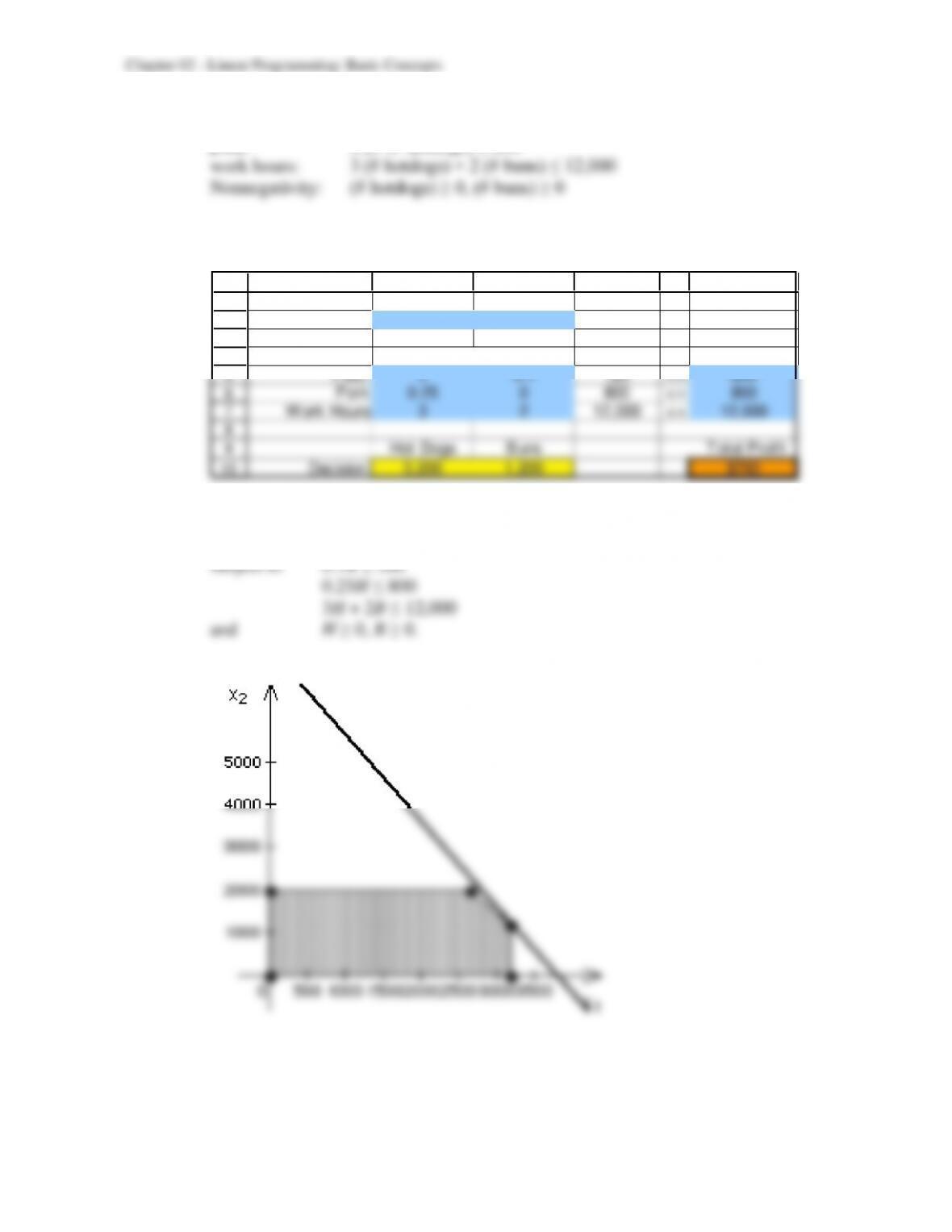
2-17
b) flour: 0.1 (# buns) ≤ 200
pork: 0.25 (# hotdogs) ≤ 800
Profit = 0.2 (# hotdogs) + 0.1 (# buns)
c)
1
2
3
4
5
6
7
8
9
10
A B C D E F
Hot Dogs Buns
Unit Profit $0.20 $0.10
Resource Resource
Used Available
Flour 0 0.1 120 <= 200
Pork 0.25 0 800 <= 800
Work Hours 3 2 12,000 <= 12,000
Hot Dogs Buns Total Profit
Decision 3,200 1,200 $760
Resource Usage
d) Let H = # of hot dogs to produce
B = # of buns to produce
Maximize P = $0.20H + $0.10B,
e) Optimal Solution: (H, B) = (x1, x2) = (3200, 1200) and P = $760.
2-19
2.18 a)
1
2
3
4
5
6
7
8
9
10
11
12
13
14
15
16
17
18
A B C D E F G H I J K
Beef Gravy Peas Carrots Roll
Unit Cost $0.40 $0.35 $0.15 $0.18 $0.10
(per ounce)
Nutritional Data (per ounce) Total in Diet Needed Maximum
Calories 54 20 15 840 320 >= 280 <= 320
Fat Calories 19 15 0 0 10 96
Vitamin A (IU) 0 0 15 350 0 600 >= 600
Vitamin C (mg) 0 1 3 1 0 12.38 >= 10
Protein (g) 8 0 1 1 1 30 >= 30
Beef Gravy Peas Carrots Roll Total Cost
Diet (ounces) 2.94 1.47 3.11 1.58 1.82 $2.62
>=
Minimums 2
Fat Calories 96 <= 96 30% of Total Calories
Gravy 1.47 >= 1.47 50% of Beef
b) Let B = ounces of beef tips in diet,
G = ounces of gravy in diet,
P = ounces of peas in diet,
Minimize Z = $0.40B + $0.35G + $0.15P + $0.18C + $0.10R
subject to 54B + 20G + 15P + 8C + 40R ≥ 280
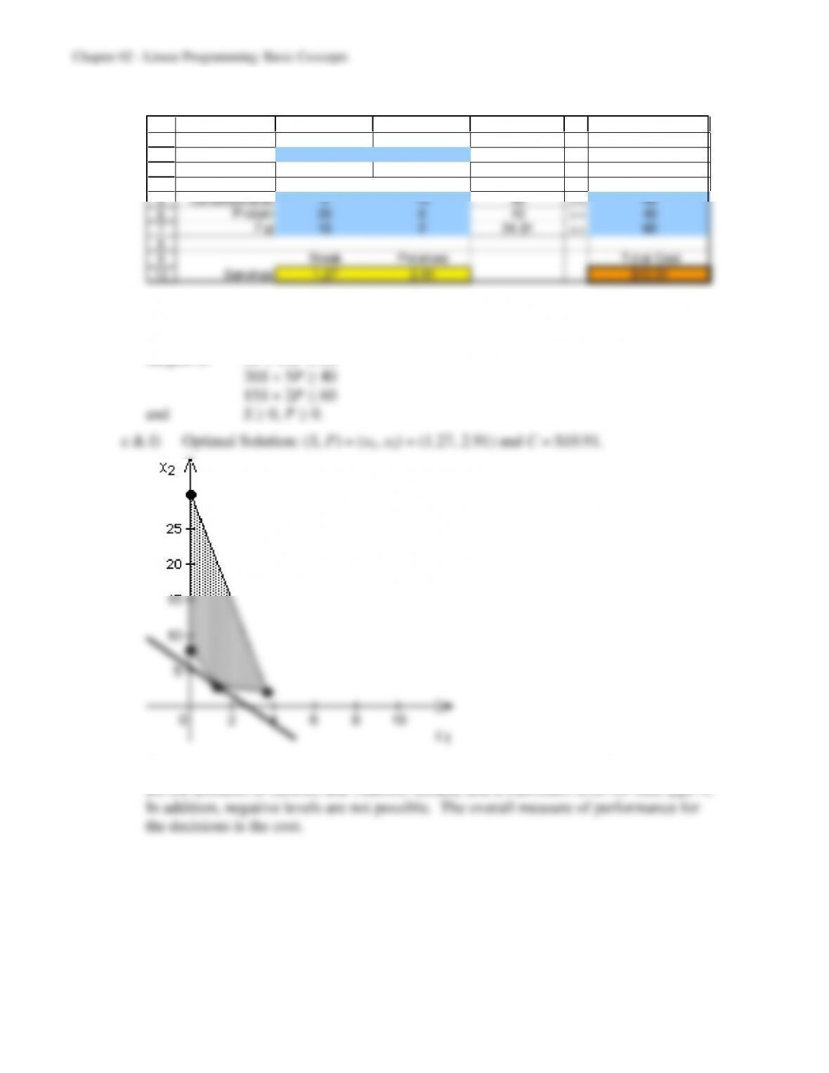
2.19 a) The decisions to be made are how many servings of steak and potatoes are needed. The
constraints are the amounts of carbohydrates, protein, and fat that are needed. In
b) carbohydrates: 5 (# steak) + 15 (# potatoes) ≥ 50
protein: 20 (# steak) + 5 (# potatoes) ≥ 40
2-20
c)
1
2
3
4
5
6
7
8
9
10
A B C D E F
Steak Potatoes
Unit Cost $4 $2
Total Nutrition Daily Requirement
(grams) (grams)
Carbohydrates 5 15 50 >= 50
Protein 20 540 >= 40
Fat 15 2 24.91 <= 60
Steak Potatoes Total Cost
Servings 1.27 2.91 $10.91
Nutritional Info (grams/serving)
d) Let S = servings of steak in diet
P = servings of potatoes in the diet
Minimize C = $4S + $2P,
subject to 5S + 15P ≥ 50
2.20 a) The decisions to be made are what combination of feed types to use. The constraints
are the amounts of calories and vitamins needed, and a maximum level for feed type A.