c)
1
2
3
4
5
6
7
8
9
10
11
12
13
14
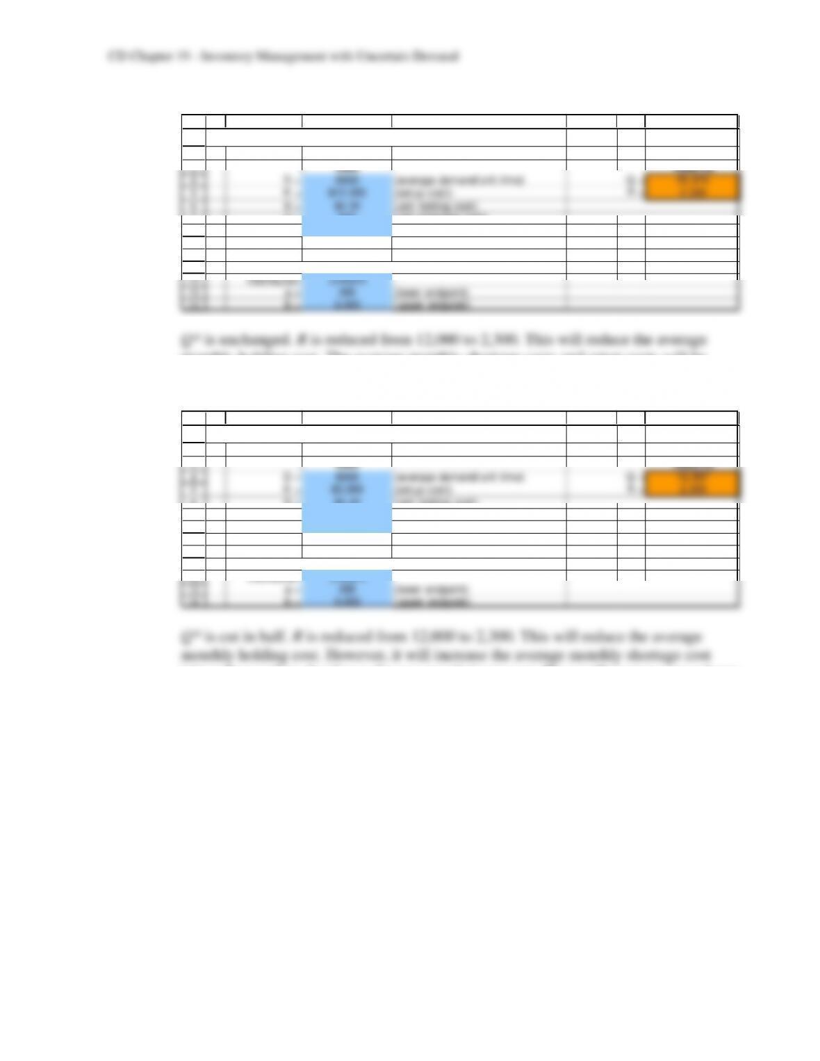
A B C D E F G
Template for the Stable Products Model
Data Results
D = 8000 (average demand/unit time) Q = 25,675
K = $12,000 (setup cost) R = 2,300
h = $0.30 (unit holding cost)
p = $10 (unit shortage cost)
L = 0.75 (service level)
Demand During Lead Time
Distribution Uniform
a = 200 (lower endpoint)
b = 3,000 (upper endpoint)
Q* is unchanged. R is reduced from 12,000 to 2,300. This will reduce the average
monthly holding cost. The average monthly shortage costs and setup costs will be
unchanged.
d)
1
2
3
4
5
6
7
8
9
10
11
12
13
14
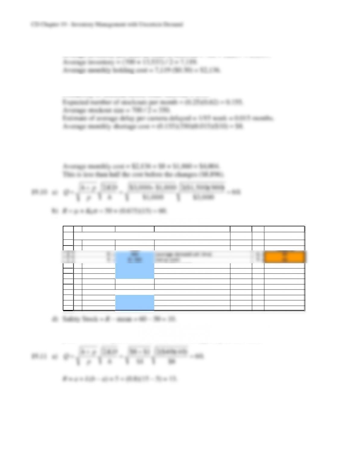
b = 3,000 (upper endpoint)
A B C D E F G
Template for the Stable Products Model
Data Results
D = 8000 (average demand/unit time) Q = 12,837
K = $3,000 (setup cost) R = 2,300
h = $0.30 (unit holding cost)
p = $10 (unit shortage cost)
L = 0.75 (service level)
Demand During Lead Time
Distribution Uniform
a = 200 (lower endpoint)
(since the number of order cycles per month increases). The smaller setup cost reduces
the average monthly setup cost.
e) Average inventory just before an order is received = 2,300 – 1,600 = 700.
Average inventory just after an order is received = 700 + 12,837 = 13,537.
Average number of orders per year = (8,000) / (12,837) = 0.62.
Probability of stockout before order received = 0.25.
Average number of setups per month = 8000 / 12,837 = 0.62.
Average monthly setup cost = (0.62)($3,000) = $1,860.
CD19-15
b)
1
2
3
4
5
6
7
8
9
10
11
12
13
14
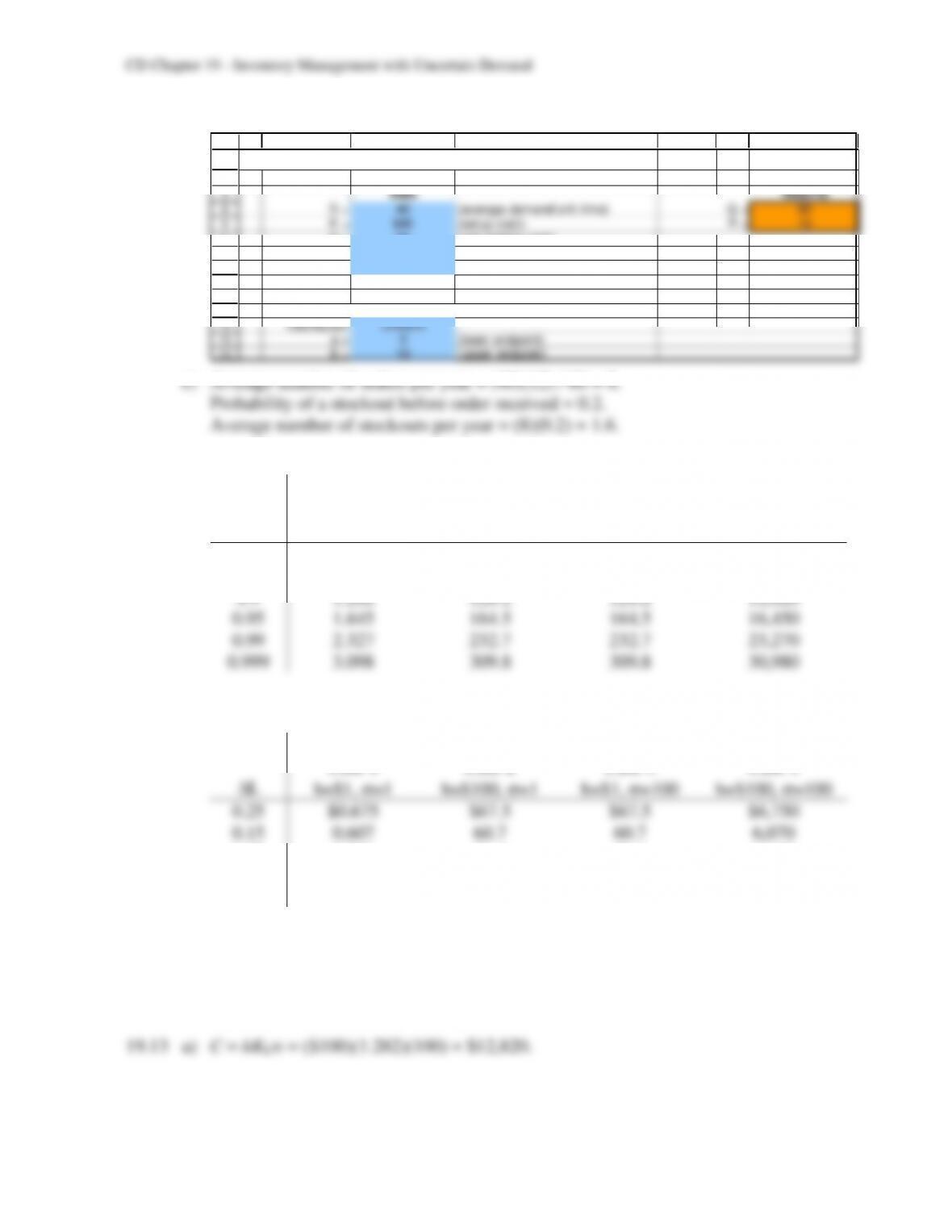
A B C D E F G
Template for the Stable Products Model
Data Results
D = 40 (average demand/unit time) Q = 60
K = $40 (setup cost) R = 13
h = $8 (unit holding cost)
p = $1 (unit shortage cost)
L = 0.8 (service level)
Demand During Lead Time
Distribution Uniform
a = 5 (lower endpoint)
b = 15 (upper endpoint)
c) Average number of orders per year = (40)(12) / 60 = 8.
Probability of a stockout before order received = 0.2.
Average number of stockouts per year = (8)(0.2) = 1.6.
19.12 a)
C = hKL
L
Case 1
h=$1, =1
Case 2
h=$100, =1
Case 3
h=$1, =100
Case 4
h=$100, =100
0.5
$0
$0
$0
$0
0.75
0.675
67.5
67.5
6,750
0.9
1.282
128.2
128.2
12,820
0.95
1.645
164.5
164.5
16,450
0.99
2.327
232.7
232.7
23,270
0.999
3.098
309.8
309.8
30,980
b)
∆C
∆L
Case 1
h=$1, =1
Case 2
h=$100, =1
Case 3
h=$1, =100
Case 4
h=$100, =100
0.25
$0.675
$67.5
$67.5
$6,750
0.15
0.607
60.7
60.7
6,070
0.05
0.363
36.3
36.3
3,630
0.04
0.682
68.2
68.2
6,820
0.009
0.771
77.1
77.1
7,710
c) As the service level gets higher, increasing the service level further costs more for
smaller increases. Thus, there will be diminishing returns when raising the service level
further and further. You should balance the cost of the safety stock with the cost of
stockouts to determine the best service level.
d) The lead time would need to quadruple to 16 days.
19.14 a) The safety stock would drop to zero.
d) The safety stock increases.
e) The safety stock doubles.
f) The safety stock doubles.
19.15 a) Ground Chuck:
1
2
3
4
5
6
7
8
9
10
11
12
13
14
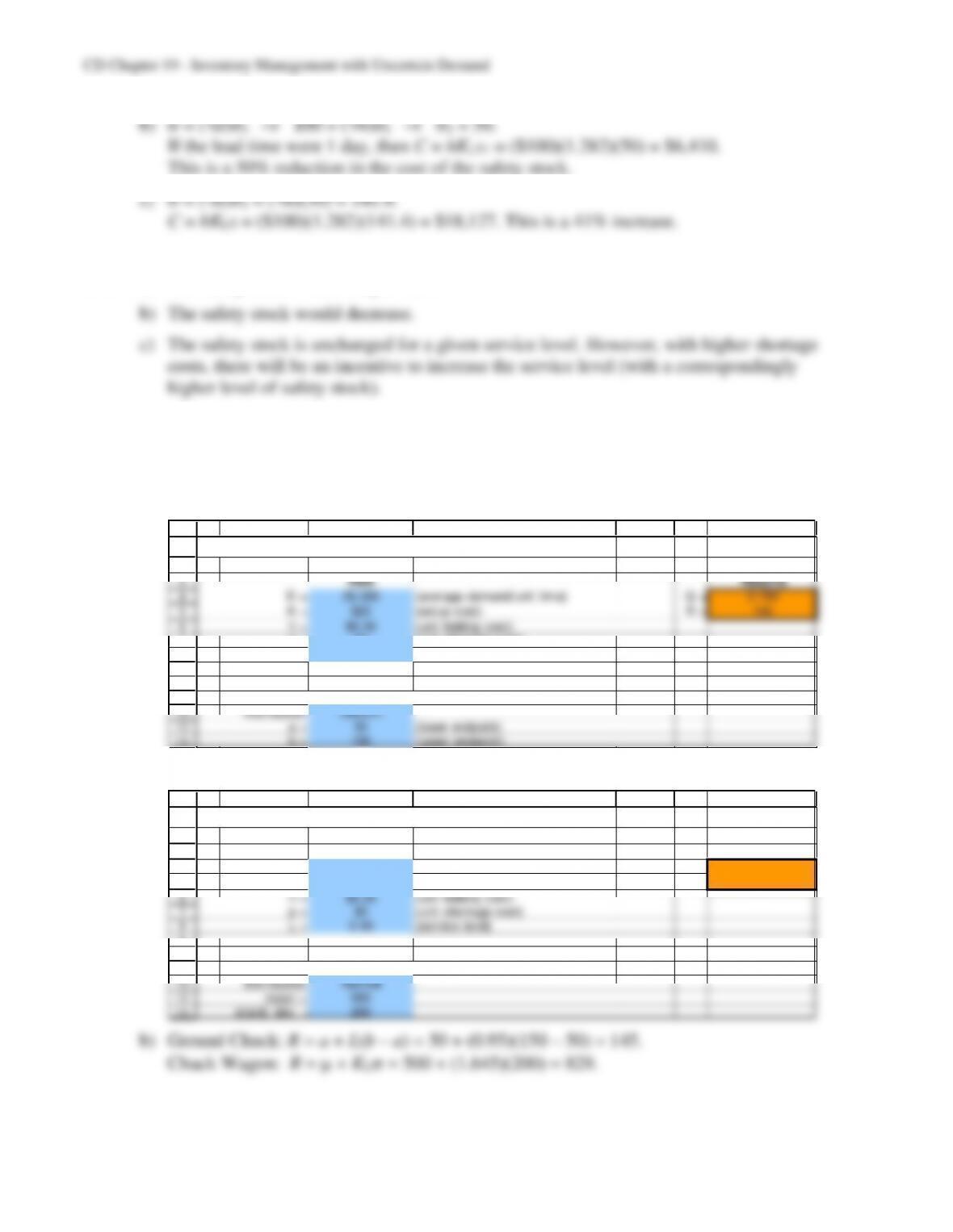
A B C D E F G
Template for the Stable Products Model
Data Results
D = 26,000 (average demand/unit time) Q = 2,183
K = $25 (setup cost) R = 145
h = $0.30 (unit holding cost)
p = $3 (unit shortage cost)
L = 0.95 (service level)
Demand During Lead Time
Distribution Uniform
a = 50 (lower endpoint)
b = 150 (upper endpoint)
Chuck Wagon:
1
2
3
4
5
6
7
8
9
10
11
12
13
14
A B C D E F G
Template for the Stable Products Model
Data Results
D = 26,000 (average demand/unit time) Q = 6,175
K = $200 (setup cost) R = 829
h = $0.30 (unit holding cost)
p = $3 (unit shortage cost)
L = 0.95 (service level)
Demand During Lead Time
Distribution Normal
mean = 500
stand. dev. = 200
b) Ground Chuck: R = a + L(b – a) = 50 + (0.95)(150 – 50) = 145.
CD19-17
e) Ground Chuck:
Annual shipping cost = K(D/Q) = ($25)(26,000 / 2,183) = $298.
Annual purchase cost = Dp = (26,000)($1.35) = $35,100.
Average annual acquisition cost = $3,442 + $35,100 = $38,542.
Jed should choose Ground Chuck as their supplier.
CD19-18
19.16. a) Option 1:
1
2
3
4
5
6
7
8
9
10
11
12
13
14
A B C D E F G
Template for the Stable Products Model
Data Results
D = 26,000 (average demand/unit time) Q = 1,093
K = $130 (setup cost) R = 366
h = $6 (unit holding cost)
p = $100 (unit shortage cost)
L = 0.99 (service level)
Demand During Lead Time
Distribution Normal
mean = 250
stand. dev. = 50
Option 2:
1
2
3
4
5
6
7
8
9
10
11
12
13
14
A B C D E F G
Template for the Stable Products Model
Data Results
D = 26,000 (average demand/unit time) Q = 678
K = $50 (setup cost) R = 995
h = $6 (unit holding cost)
p = $100 (unit shortage cost)
L = 0.99 (service level)
Demand During Lead Time
Distribution Uniform
a = 500 (lower endpoint)
b = 1,000 (upper endpoint)
b) Option 1: R = + KL = 250 + (2.327)(50) = 366.
e) Option 1:
Option 2:
CD19-19
Cases
19.1 For the analysis of this case we use the template for perishable products.
1
2
3
4
5
6
A B C D E F
Optimal Service Level for Perishable Products
Data Results
Unit Sales Price $5 Cost of Overordering $2
Unit Purchase Cost $3 Cost of Underordering $2
Unit Salvage Value $1 Optimal Service Level 0.5
Since Talia assumes that demand is normally distributed, we must estimate the
parameters for the demand distribution. The mean is 250 firecracker sets. The standard
deviation can be approximated by examining the lowest and highest selling stands from
sets.
CD19-20
b) If Leisure Limited refunds 75% of the purchase cost, then the unit salvage value for a
1
2
3
4
5
6
A B C D E F
Optimal Service Level for Perishable Products
Data Results
Unit Sales Price $5 Cost of Overordering $1
Unit Purchase Cost $3 Cost of Underordering $2
Unit Salvage Value $1.75 Optimal Service Level 0.615
From the normal table, Howie should order 0.3 above the mean to attain a service
For the case of a 25% refund the unit salvage value equals $0.25.
1
2
3
4
5
6
A B C D E F
Optimal Service Level for Perishable Products
Data Results
Unit Sales Price $5 Cost of Overordering $3
Unit Purchase Cost $3 Cost of Underordering $2
Unit Salvage Value $0.25 Optimal Service Level 0.421
From the normal table, Howie should order 0.2 below the mean to attain a service
c) For a unit sale price of $6 and a 50% refund on returned firecracker sets, the optimal
service level can be determined as follows:
1
2
3
4
5
6
A B C D E F
Optimal Service Level for Perishable Products
Data Results
Unit Sales Price $6 Cost of Overordering $2
Unit Purchase Cost $3 Cost of Underordering $3
Unit Salvage Value $1 Optimal Service Level 0.6
However, if Howie raises the price of a firecracker set, one would expect that the
demand for his sets will decrease. Therefore, Talia should not use the same demand
distribution that she used for her previous calculations of the optimal order quantity.
CD19-21
d) Talia’s strategy for estimating the demand is overly simplistic. She makes the
simplifying assumption that the demand is normally distributed. However, she does not
Talia should also reevaluate her assumption that the demand is normally distributed.
She should check how her forecasts change if she uses other demand distributions.
19.2 a) We can use the statistical functions in Excel to compute the sample mean and sample
variance:
1
2
3
4
5
6
7
8
9
10
11
12
13
14
15
16
17
18
19
A B
Number of
Month MX332 o rdered
June 25
July 31
August 18
September 22
October 40
November 19
December 38
January 21
February 25
March 36
April 34
May 28
June 27
Mean = 28
St. Dev. = 7.3
Variance = 53.2
The sample mean is 28 and the sample variance is 53.2.
b) The mean lead time is one month. The stated worst-case scenario is that the “delivery
CD19-22
c) Based on the findings of Scarlett Windermere, American Aerospace can use a (R, Q)
policy for the inventory of part 10003487. The assumptions of this model are satisfied:
1. The part is a stable product.
2. Its inventory level is under continuous review.
3. While the production of this part itself has no lead time, it is typically delayed by the
Note that the average demand per year equals D = 12*28 = 336. The average demand
during the lead time equals 1*28 = 28, and its variance and standard deviation are
1
2
3
4
5
6
7
8
9
10
11
12
13
14
A B C D E F G
Template for the Stable Products Model
Data Results
D = 336 (average demand/unit time) Q = 80
K = $5,800 (setup cost) R = 37
h = $750 (unit holding cost)
p = $3,250 (unit shortage cost)
L = 0.85 (service level)
Demand Du ring Lead Time
Distribution Normal
mean = 28
stand. dev. = 8.7
American Aerospace should implement an (R, Q) policy with R = 37 and Q = 80.
CD19-23
1
2
3
4
5
6
7
8
9
10
11
12
13
14
A B C D E F G
Template for the Stable Products Model
Data Results
D = 336 (average demand/unit time) Q = 80
K = $5,800 (setup cost) R = 42
h = $750 (unit holding cost)
p = $3,250 (unit shortage cost)
L = 0.95 (service level)
Demand Du ring Lead Time
Distribution Normal
mean = 28
stand. dev. = 8.7
The average inventory just before an order arrives equals 42 – 28 = 14, and just after
f) Scarlett’s independent analysis of the stationary part 10003487 can only be justified
since there is only a single jet engine that needs this part, and this part appears to be the
bottleneck in the production process. But more often, the same stationary part will be
used for several jet engines. As a result the demand for stationary parts will depend on
g) Scarlett could try to forecast the demand for jet engines based on sales data from
previous years.