
CD19-1
CD Chapter 19 Inventory Management with Uncertain Demand
Review Questions
19.1-1 Freddie should consider the trade-off between too much inventory and too little
inventory.
19.1-2 Based on Freddie’s data, 9, 10, and 11 are the only numbers of copies that he has sold in
the past.
19.2-3 It is assumed that the demand during the period is uncertain but that the probability
distribution of demand is known.
19.2-5 Bayes’ decision rule will make the same decision since both approaches are applying
Bayes’ decision rule, but with different payoffs, where one is to be maximized and the
other minimized.
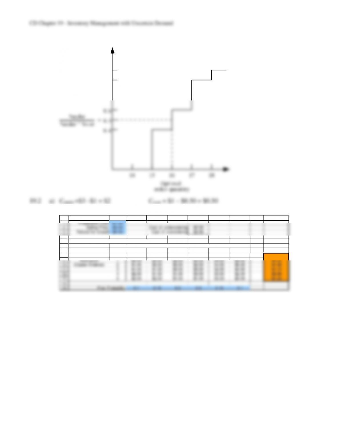
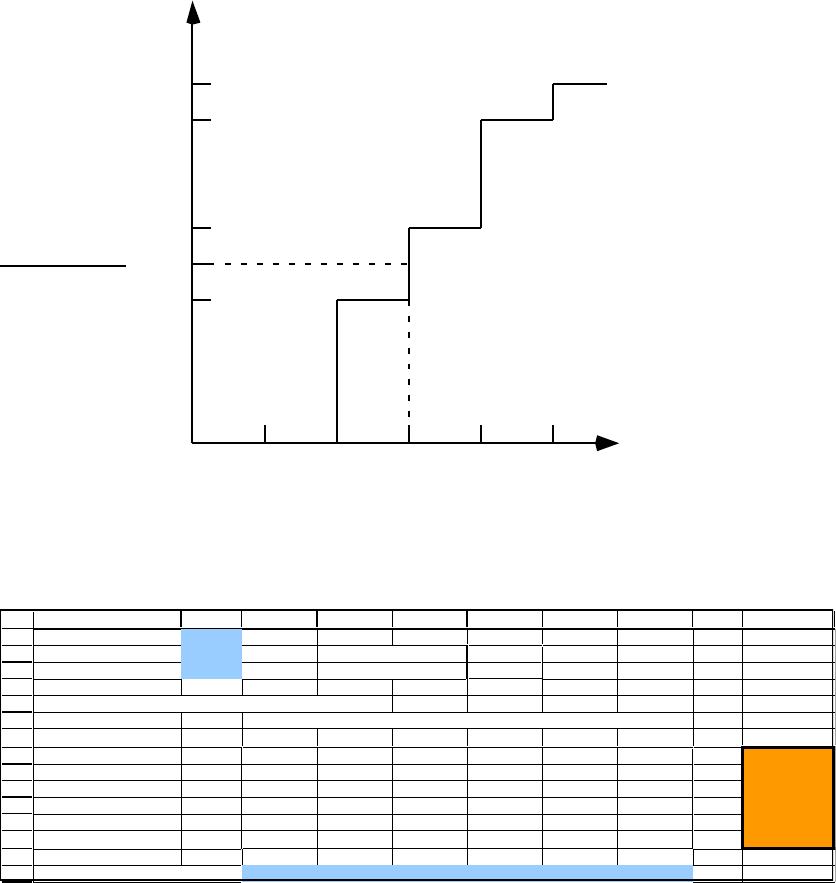
19.2-8 The point at which the optimal service level hits the cumulative distribution function
gives the optimal order quantity.
19.2-9 Yes.
19.3-1 There have been four stockouts of panoramic disposable cameras during the year with
durations ranging from a few days to a couple weeks.
19.3-3 The Division Vice President for Production is concerned about the frequent interruptions
in the production of other models caused by setting up for a production run for the
disposable panoramic cameras. He is recommending having much longer production
runs much less frequently.
CD19-2
19.3-4 The Division President is skeptical about his Vice President’s recommendation because it
would increase inventory levels. He has been promoting the just-in-time philosophy of
minimizing inventory.
19.4-2 Under the old inventory policy, the probability of a stockout is 50% and the maximum
size of a stockout is 8,000.
19.4-5 Management made the decision on how much safety stock to provide.
19.4-6 The relevant cost factors for choosing the order quantity are acquisition costs, setup costs,
holding costs, and shortage costs.
19.4-8 Increasing the order quantity decreases the average monthly setup costs because this
decreases the average number of setups required per month. Increasing the order
19.4-9 The management science team used the EOQ model with planned shortages to find the
approximately optimal order quantity.
19.4-11 The high setup cost, the long lead time, and the high variability in monthly sales were the
three factors the caused the cost of this inventory policy to be unusually high.
19.4-12 The setup cost and lead time will be greatly reduced by acquiring some additional
production facilities that would be used solely for production of the disposable panoramic
cameras.
CD19-3
19.5-3 The traditional method of implementing a continuous-review inventory system was to use
a two-bin system.
19.5-5 An (R, Q) inventory policy controls a continuous-review inventory system by using a
fixed reorder point R and a fixed order quantity Q.
19.5-7 The EOQ model with planned shortages is used to approximate the optimal order
quantity.
19.5-9 The most convenient measure of the service level is the probability that a stockout will
not occur between the time an order is placed and the order quantity is received.
19.5-10 R = + KL.
19.6-2 Occasionally it is not appropriate to apply a single-product inventory model because of
interactions between the products.
19.6-3 A multiechelon inventory system is a system with multiple echelons of inventory where
each echelon (except the bottom one) is used to replenish the inventories at the various
sites of the next lower echelon.
19.6-5 The three factors that proved to be especially important were the inclusion of a user team
as advisors to the project team, a very extensive user acceptance test whereby users could
CD19-4
19.6-8 HP faced inventories mounting into the billions of dollars and alarming customer
dissatisfaction with its order fulfillment process.
19.6-10 A key intangible benefit was to enhance HP’s reputation as a progressive company that
can be counted on by its customers to fill their orders promptly.
CD19-5
Problems
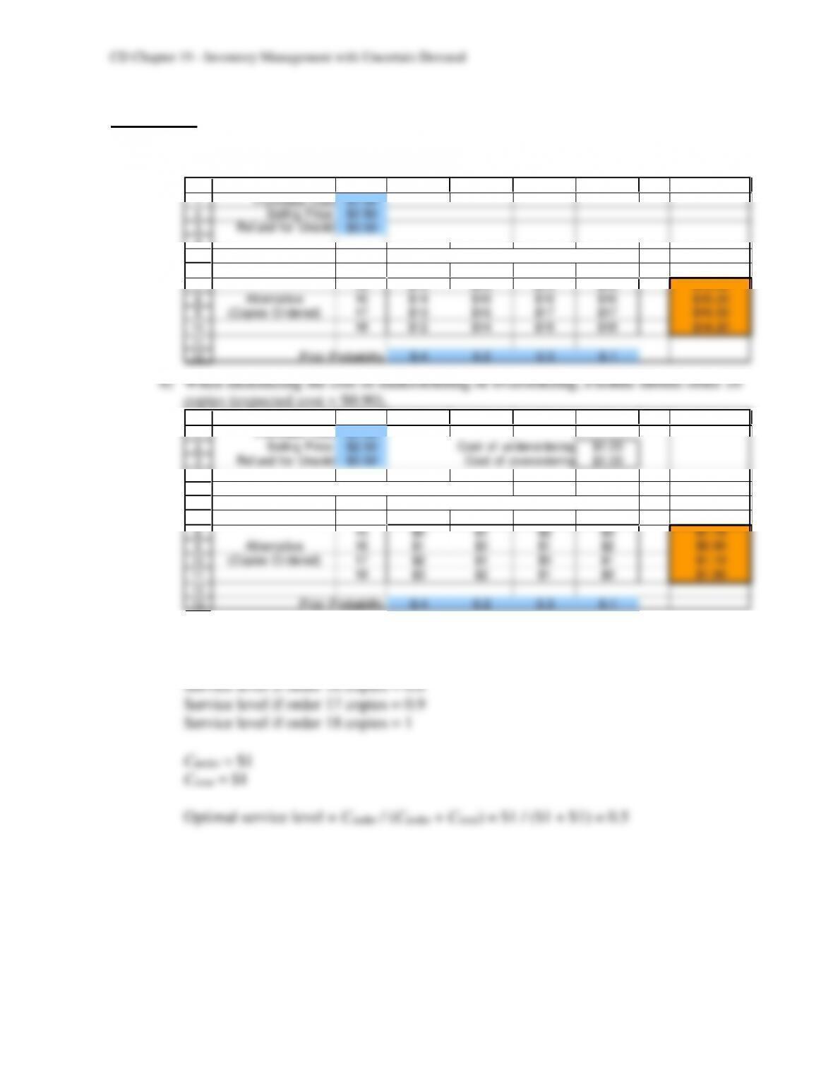
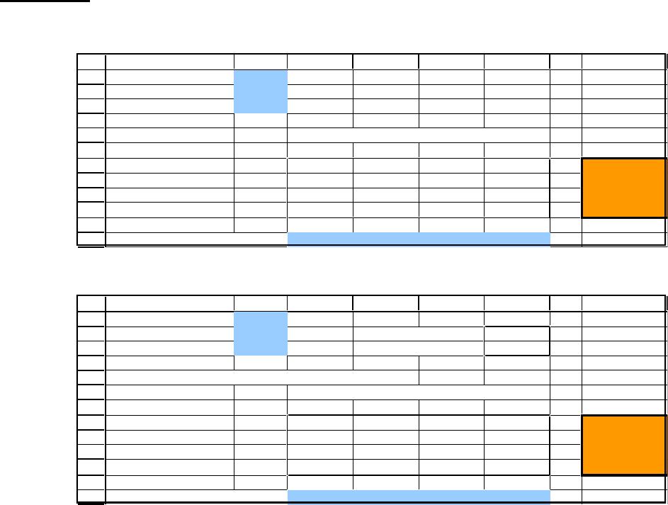
19.1 a) When maximizing profit, Freddie should order 16 copies (expected profit = $15.20).
4
5
6
7
9
A B C D E F G H
Payoff Table Expected
15 16 17 18 Profit
State of Nature (Purchase Requests)
1
3
4
5
6
7
9
A B C D E F G H
Purchase Cost $1.50
Cost of Overordering + Cost of Underordering
Expected
15 16 17 18 Cost
State of Nature (Purchase Requests)
Freddie’s most profitable alternative is to order 16 copies.
c) Service level if order 15 copies = 0.4
Freddie should order 16 copies.
CD19-6
d)
P(de mand Š x)
0. 9
1
b)
1
2
3
4
5
6
7
8
9
A B C D E F G H I J
Cost of Overordering + Cost of Underordering
Expected
0 1 2 3 4 5 Cost
0 $0.00 $2.00 $4.00 $6.00 $8.00 $10.00 $5.10
3 $1.50 $1.00 $0.50 $0.00 $2.00 $4.00 $1.10
4 $2.00 $1.50 $1.00 $0.50 $0.00 $2.00 $0.98
State of Nature (Purchase Requests)
Prepare 4 doughnuts each day to minimize costs.
CD19-7
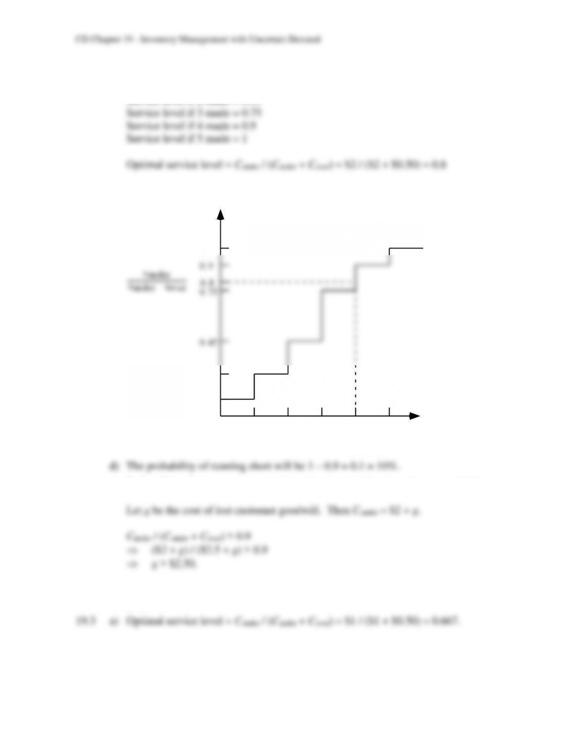
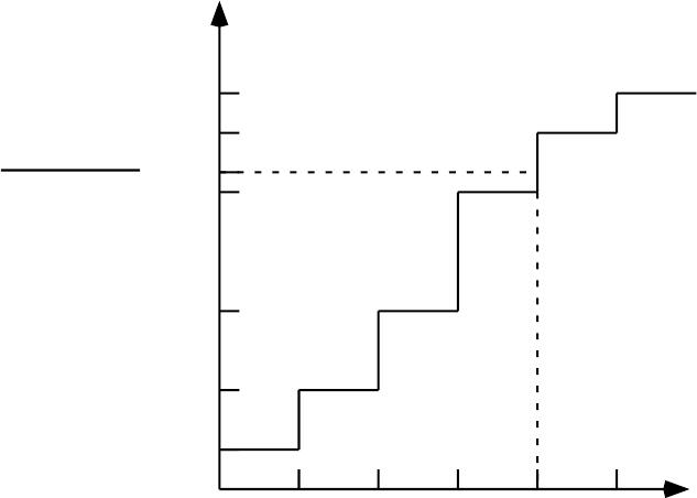
c) Service level if 0 made = 0.1
Service level if 1 made = 0.25
Service level if 2 made = 0.45
Prepare 4 doughnuts each day.
P(de ma nd Š x)
0. 1
1
0. 25
1 2 3 4 5
Opti ma l
orde r qua ntit y
e) Before 5 doughnuts are prepared, the optimal service level needs to exceed 0.9.
The goodwill cost would need to be at least $2.50 before 5 doughnuts should be
prepared.
CD19-8
b)
P(de mand Š x)
1
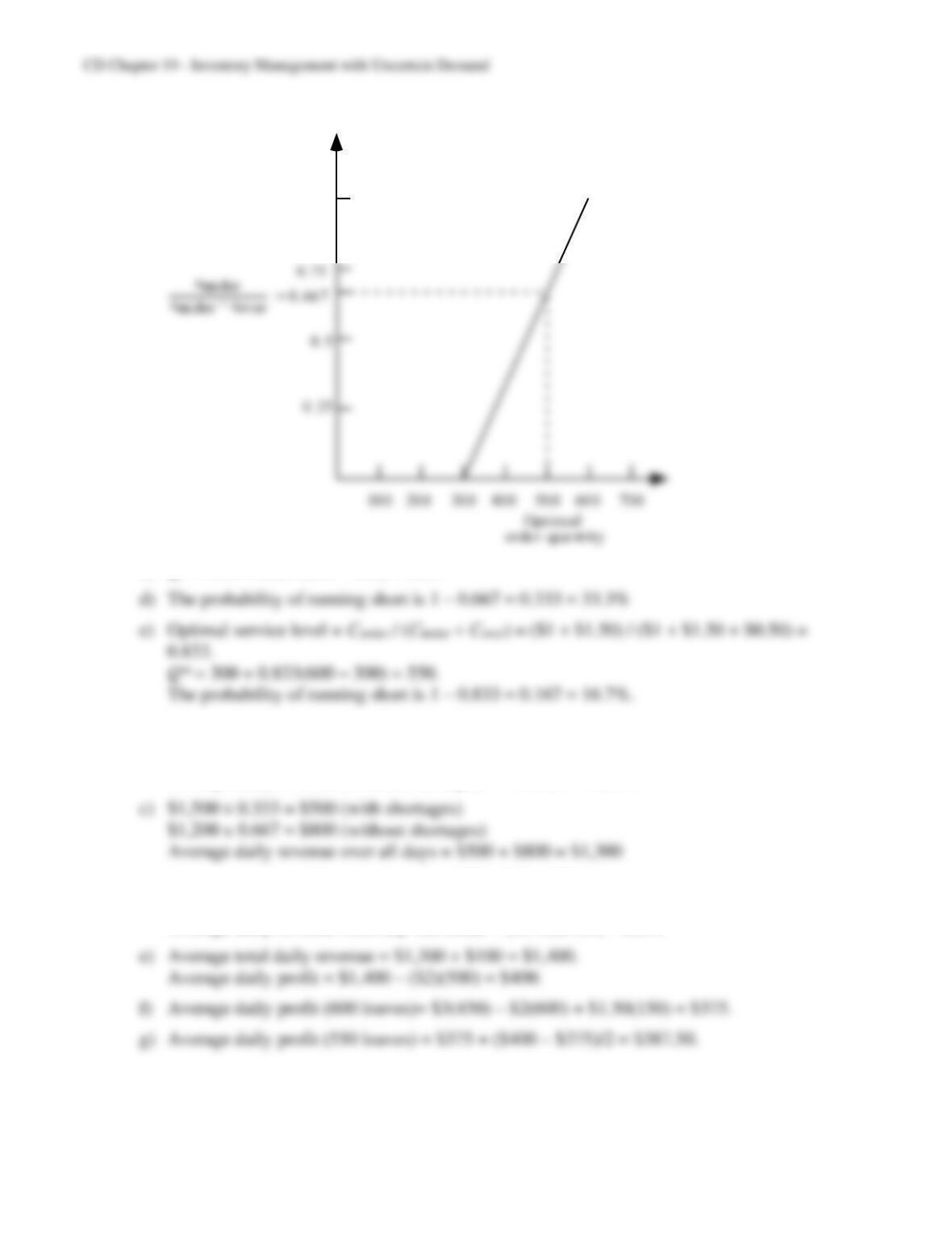
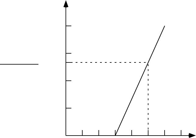
c) Q* = 300 + 0.667(600 – 300) = 500.
19.4 a) Revenue (with shortages) = 500($3) = $1,500
b) Average number of loaves sold (without shortages) = 300 + (500–300)/2 = 400.
Average daily revenue (without shortages) = 400($3) = $1,200.
d) Average number of loaves not sold = (200–0)/2 = 100.
Average number of day-old loaves obtained over all days = 100 x 0.667 = 66.7.
Average daily revenue from day-old bread = (66.7)($1.50) = $100.
CD19-9
i) Average size of shortage (500 loaves) = (100 – 0)/2 = 50 loaves.
Average daily shortage over all days = (50)(0.333) = 16.67.
b) Probability of incurring shortage = 1 – 0.667 = 33.3% which is the same as in problem
19.3.
The corresponding numbers for problem 19.3 are 100 and 200 respectively which are
four times the amounts here.
d) The average daily costs of underordering and overordering for the new plan are 25% of
the original costs. Thus, it is quite valuable to obtain as much information as possible
about demand before placing the final order for a perishable product.
19.6 a) This problem can be interpreted as an inventory problem with uncertain demand for a
perishable product with traveler’s checks as the product. Once Stan gets back from his
CD19-10
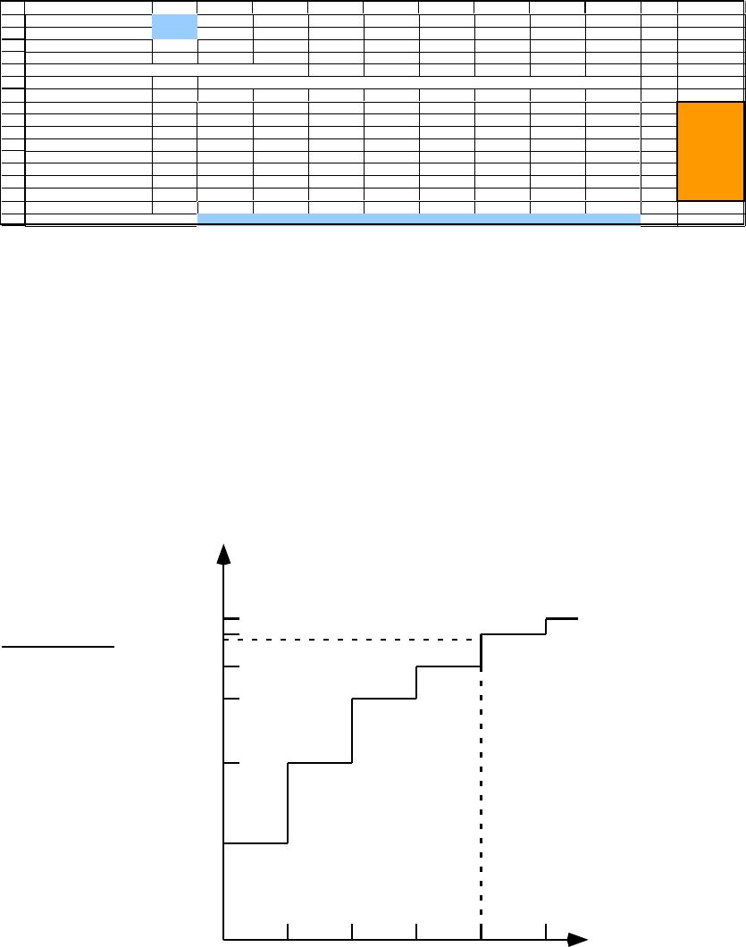
b)
1
2
3
4
5
6
7
8
A B C D E F G H I J K L
Cost of underordering $49
Cost of overordering $3
Cost of Overordering + Cost of Underorderin g
Expected
10 11 12 13 14 15 16 17 Cost
10 $0 $49 $98 $147 $196 $245 $294 $343 $166.60
State of Nature ($100 Traveler’s Checks Needed)
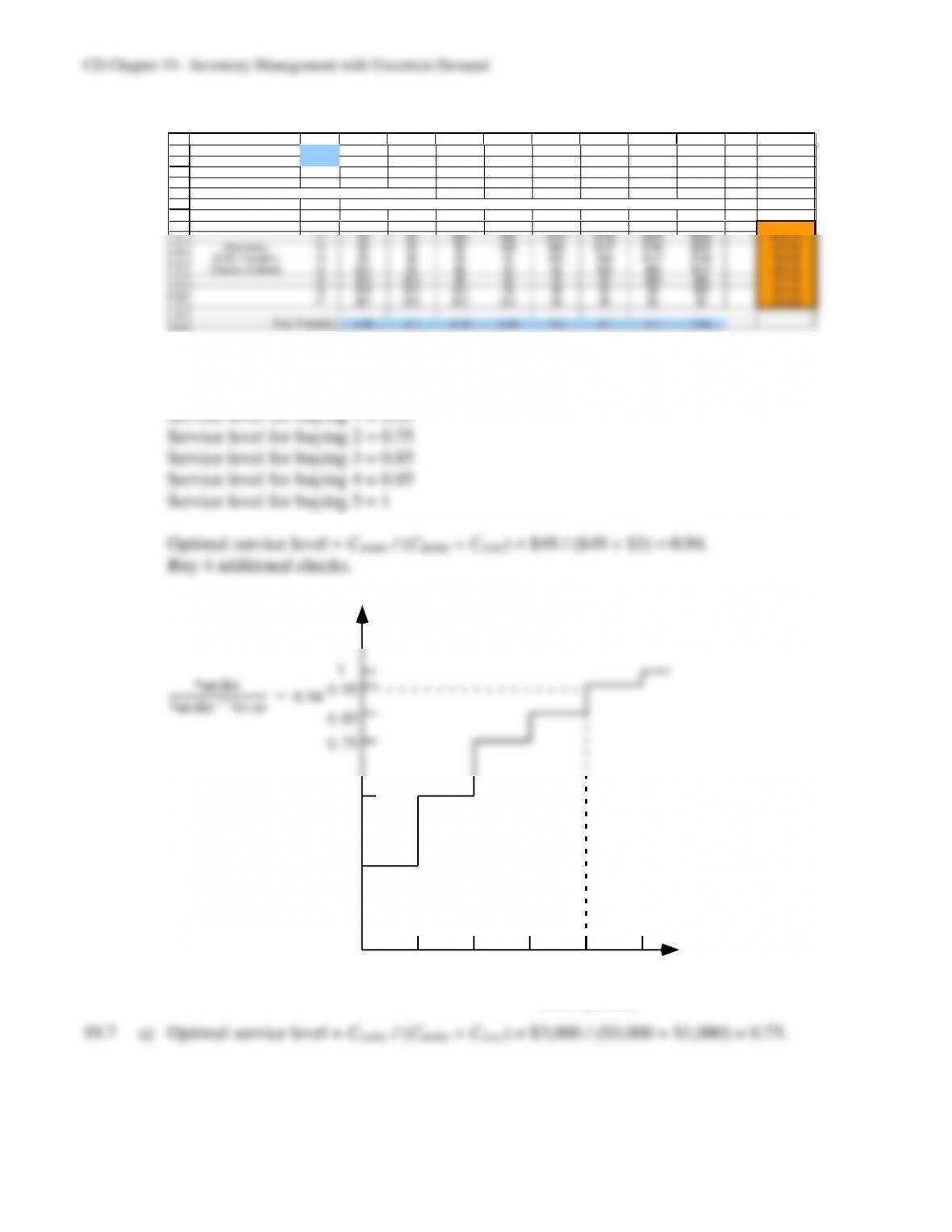
Purchase 4 additional $100 checks, for a total of $1,600.
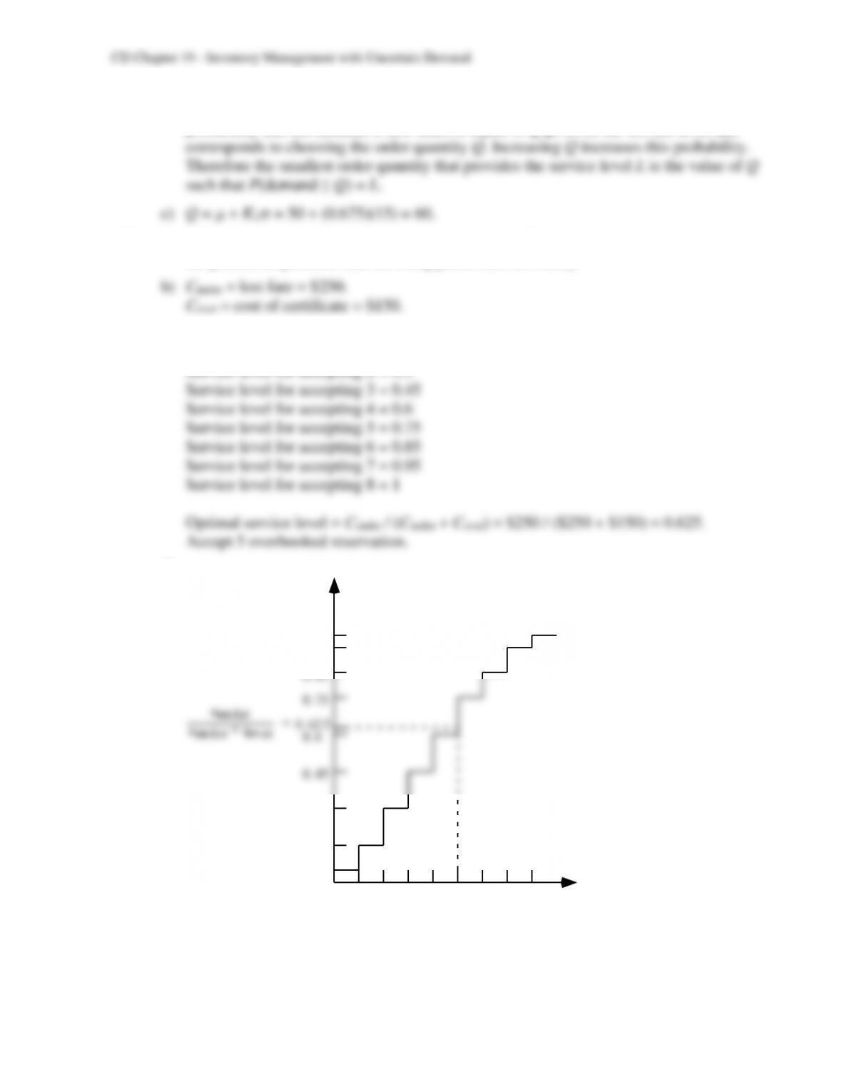
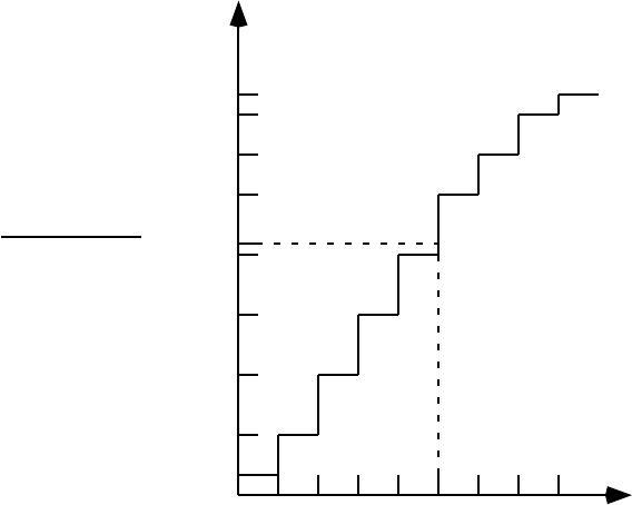
c) Service level for buying 0 = 0.3
d)
P(de m and Š x)
0. 55
0. 3
1 2 3 4 5
Opti m al
orde r qua nt it y
CD19-11
b) When the demand is less-than-or-equal-to Q, no shortage will occur. Therefore the
probability that the demand is less-than-or-equal-to Q gives us the service level that
19.8 a) When interpreting this problem as an inventory problem, overbooked reservations are
the perishable products that are being placed into inventory.
c) Service level for accepting 0 = 0.05
Service level for accepting 1 = 0.15
d)
P(de mand Š x)
0. 15
0. 3
1
0. 05
1 2 3 4 5
Opti mal
orde r quant it y
6 7 8
0. 95
CD19-12
19.9 a)
1
6
9
10
A B C D E F G
Template for the Stable Products Model
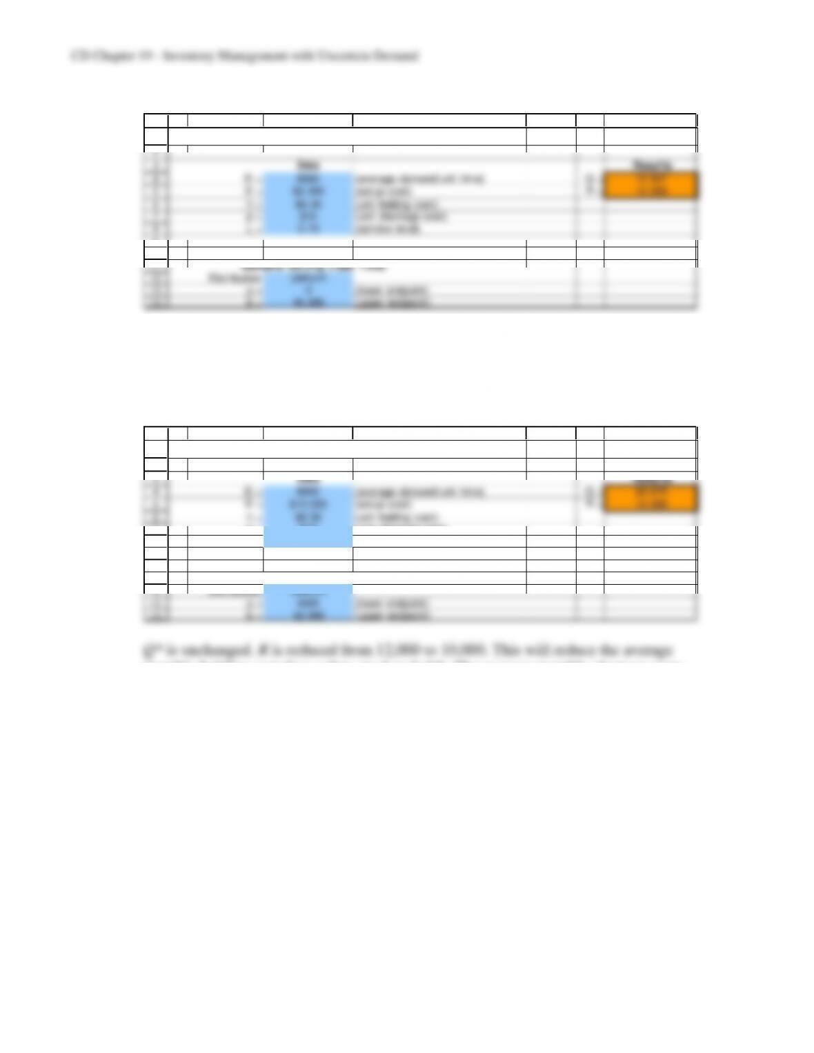
Q* is cut in half. R is unchanged. This will reduce the average monthly holding cost.
However, it will increase the average monthly shortage cost (since the number of order
cycles per month increases). The smaller setup cost reduces the average monthly setup
cost.
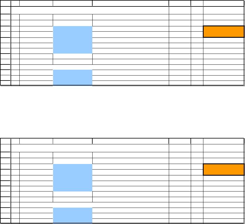
b)
1
2
4
6
7
8
9
10
11
14
A B C D E F G
Template for the Stable Products Model
p = $10 (unit shortage cost)
L = 0.75 (service level)
Demand During L ead Time
monthly holding cost (less safety stock to hold). The average monthly shortage costs
and setup costs will be unchanged.