CD18-16
1
2
3
4
5
6
7
8
9
10
11
A B C D E F G
EOQ Model with Planned Shortages (Analytical Version)
Data Results
D = 6,000 (demand/year) Max Inventory Level 507
K = $115 (setup cost)
h = $4.20 (unit holding cost) Annual Setup Cost $1,064
p = $15.00 (unit shortage cost) Annual Holding Cost $831
Annual Shortage Cost $233
Decision Total Variable Cost $2,128
Q = 649 (optimal order quantity)
S = 142 (optimal maximum shortage)
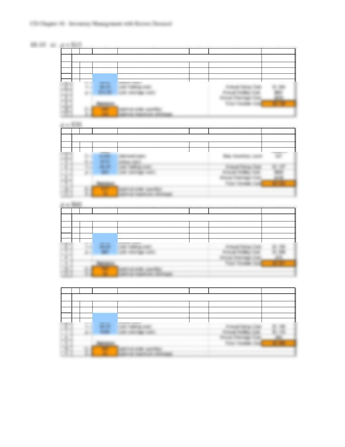
p = $30
1
2
3
4
5
6
7
8
9
10
11
A B C D E F G
EOQ Model with Planned Shortages (Analytical Version)
Data Results
D = 6,000 (demand/year) Max Inventory Level 537
K = $115 (setup cost)
h = $4.20 (unit holding cost) Annual Setup Cost $1,127
p = $30 (unit shortage cost) Annual Holding Cost $989
Annual Shortage Cost $138
Decision Total Variable Cost $2,255
Q = 612 (optimal order quantity)
S = 75 (optimal maximum shortage)
p = $60
1
2
3
4
5
6
7
8
9
10
11
A B C D E F G
EOQ Model with Planned Shortages (Analytical Version)
Data Results
D = 6,000 (demand/year) Max Inventory Level 554
K = $115 (setup cost)
h = $4.20 (unit holding cost) Annual Setup Cost $1,164
p = $60 (unit shortage cost) Annual Holding Cost $1,088
Annual Shortage Cost $76
Decision Total Variable Cost $2,327
Q = 593 (optimal order quantity)
S = 39 (optimal maximum shortage)
p = $120
1
2
3
4
5
6
7
8
9
10
11
A B C D E F G
EOQ Model with Planned Shortages (Analytical Version)
Data Results
D = 6,000 (demand/year) Max Inventory Level 563
K = $115 (setup cost)
h = $4.20 (unit holding cost) Annual Setup Cost $1,183
p = $120 (unit shortage cost) Annual Holding Cost $1,143
Annual Shortage Cost $40
Decision Total Variable Cost $2,366
Q = 583 (optimal order quantity)
S = 20 (optimal maximum shortage)
CD18-17
b)
p
TVC
% reduction from basic model
$15
$2,128
12%
$30
$2,255
6%
$60
$2,327
3%
$120
$2,366
1.5%
c)
p
Max. wait time (days)
Acceptable case
$15
5.9
$30
3.1
$60
1.6
*
$120
0.8
*
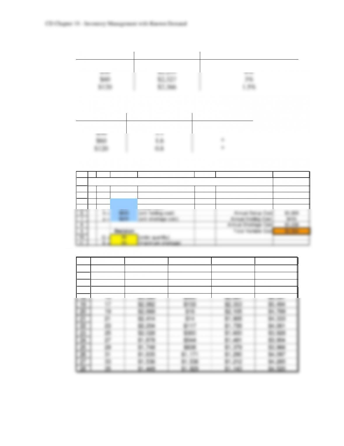
18.11 a) The TVC is reduced from $7,800 to $3,904, a reduction of $3,896 (about 50%).
1
2
3
4
5
6
7
8
9
10
11
A B C D E F G
EOQ Model with Planned Shortages (Solver Version)
Data Results
D = 676 (demand/year) Max Inventory Level 6
K = $75 (setup cost)
h = $600 (unit holding cost) Annual Setup Cost $1,950
p = $200 (unit shortage cost) Annual Holding Cost $415
Annual Shortage Cost $1,538
Decision Total Variable Cost $3,904
Q = 26 (order quantity)
S = 20 (maximum shortage)
b)
14
15
16
17
18
19
20
21
22
23
24
25
26
27
28
C D E F G
Annual Annual Annual Total
Setup Holding Shortage Variable
Q Cost Cost Cost Cost
$1,950 $415 $1,538 $3,904
15 $3,380 $500 $2,667 $6,547
17 $2,982 $159 $2,353 $5,494
19 $2,668 $16 $2,105 $4,789
21 $2,414 $14 $1,905 $4,333
23 $2,204 $117 $1,739 $4,061
25 $2,028 $300 $1,600 $3,928
27 $1,878 $544 $1,481 $3,904
29 $1,748 $838 $1,379 $3,966
31 $1,635 $1,171 $1,290 $4,097
33 $1,536 $1,536 $1,212 $4,285
35 $1,449 $1,929 $1,143 $4,520
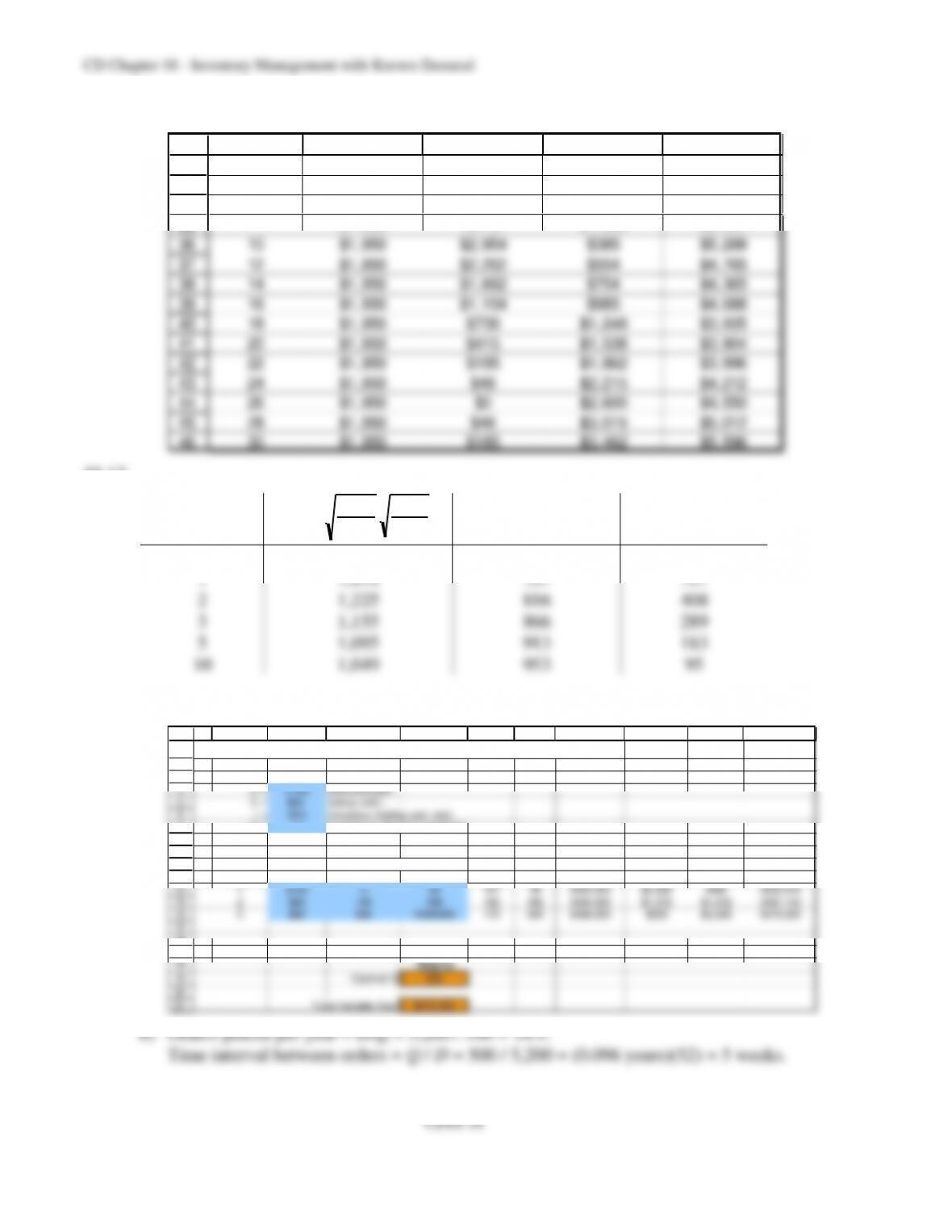
18.14 a)
1
2
3
4
5
6
7
8
9
10
11
12
13
14
15
16
17
18
19
20
21
A B C D E F G H I J K
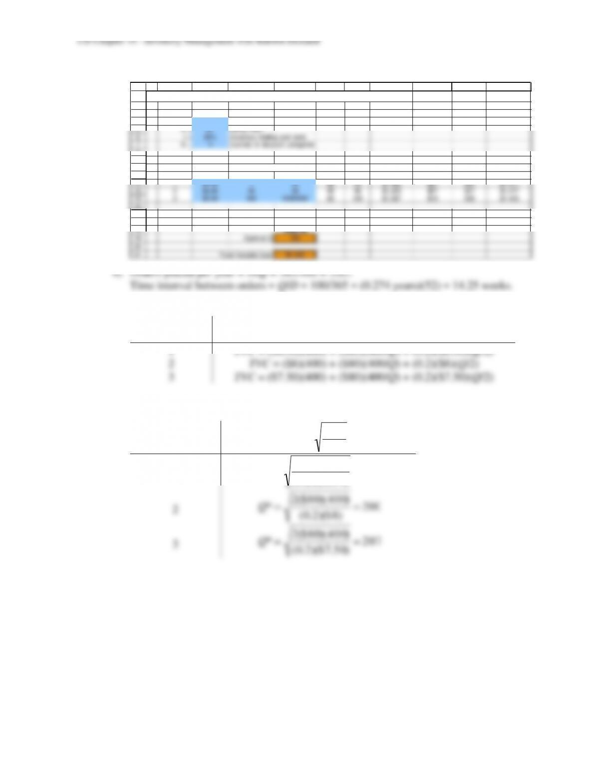
EOQ Model with Quantity Discounts (Analytical Version)
Data
D = 365 (demand/year)
K = $5 (setup cost)
I = 20% (inventory holding cost rate)
N = 3
(number of discount categories)
Annual Annual Annual T otal
Range of order quantities Purchase Setup Holding Variable
Category Price Lower Limit Upper Limit EOQ Q* Cost Cost Cost Cost
1 $4.00 1 49 68 49 $1,460 $37 $20 $1,517
2 $3.90 50 99 68 68 $1,424 $27 $27 $1,477
3 $3.80 100 10000000 69 100 $1,387 $18 $38 $1,443
Results
Optimal Q 100
Total Variable Cost $1,443
b) Orders placed per year = D/Q = 365/100 = 3.65.
Time interval between orders = Q/D = 100/365 = (0.274 years)(52) = 14.25 weeks.
18.15 a)
Discount
Category
TVC = cD + K(D/Q) = h(Q/2)
1
TVC = ($8.50)(400) + ($80)(400/Q) + (0.2)($8.50)(Q/2)
2
TVC = ($8)(400) + ($80)(400/Q) + (0.2)($8)(Q/2)
3
TVC = ($7.50)(400) + ($80)(400/Q) + (0.2)($7.50)(Q/2)
b)
Discount
Category
Q*=2KD
h
1
Q*=2($80)(400)
(0.2)($8.50)
=194
2
Q*=2($80)( 400)
(0.2)($8)
=200
3
Q*=2($80)( 400)
(0.2)($7.50)
=207
CD18-20
c)
Discount
Category
Feasible
Q
TVC = cD + K(D/Q) = h(Q/2)
1
99
$3,807
2
200
$3,520
3
1,000
$3,782
d)
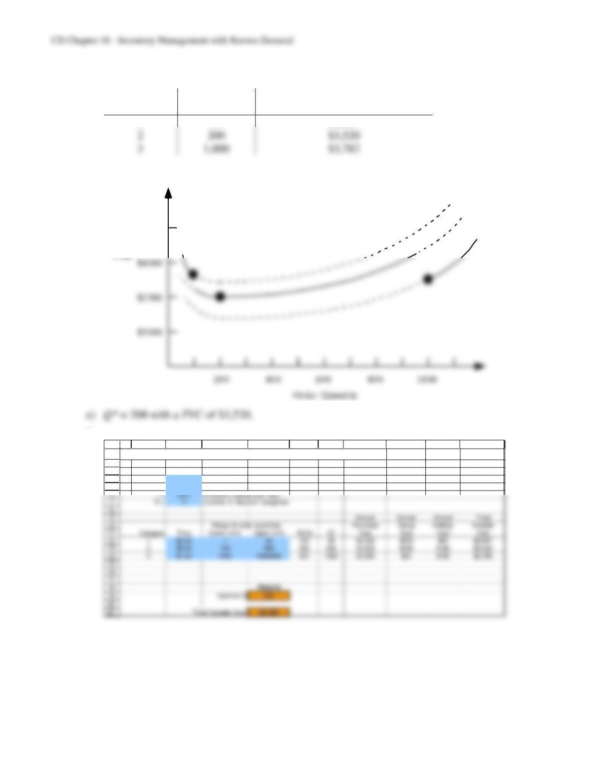
200 400
$3000
$3500
$4000
$4500
600 800 1000
Order Quanti ty
Total
Vari abl e
Cost
f)
1
2
3
4
5
6
7
8
9
10
11
12
13
14
15
16
17
18
19
20
21
A B C D E F G H I J K
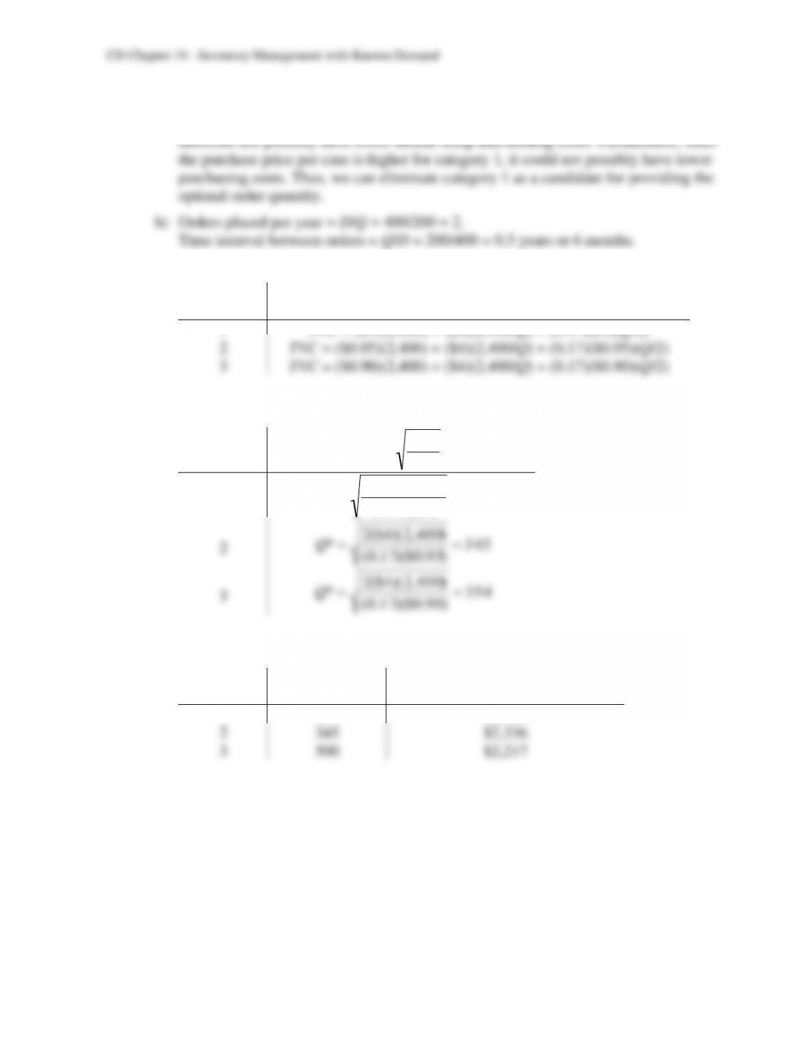
EOQ Model with Quantity Discounts (Analytical Version)
Data
D = 400 (demand/year)
K = $80 (setup cost)
I = 20% (inventory holding cost rate)
N = 3
(number of discount categories)
Annual Annual Annual T otal
Range of order quantities Purchase Setup Holding Variable
Category Price Lower Limit Upper Limit EOQ Q* Cost Cost Cost Cost
1 $8.50 1 99 194 99 $3,400 $323 $84 $3,807
2 $8.00 100 999 200 200 $3,200 $160 $160 $3,520
3 $7.50 1000 10000000 207 1000 $3,000 $32 $750 $3,782
Results
Optimal Q 200
Total Variable Cost $3,520
CD18-21
g) Since the value of Q that minimizes TVC for discount category 2 is feasible that means
that this order quantity minimizes the annual setup and holding costs. Category 1 could
18.16 a)
Discount
Category
TVC = cD + K(D/Q) = h(Q/2)
1
TVC = ($1)(2,400) + ($4)(2,400/Q) + (0.17)($1)(Q/2)
2
TVC = ($0.95)(2,400) + ($4)(2,400/Q) + (0.17)($0.95)(Q/2)
3
TVC = ($0.90)(2,400) + ($4)(2,400/Q) + (0.17)($0.90)(Q/2)
b)
Discount
Category
Q*=2KD
h
1
Q*=2($4)(2,400)
(0.17)($1)
=336
2
Q*=2($4)(2,400)
(0.17)($0.95)
=345
3
Q*=2($4)(2,400)
(0.17)($0.90)
=354
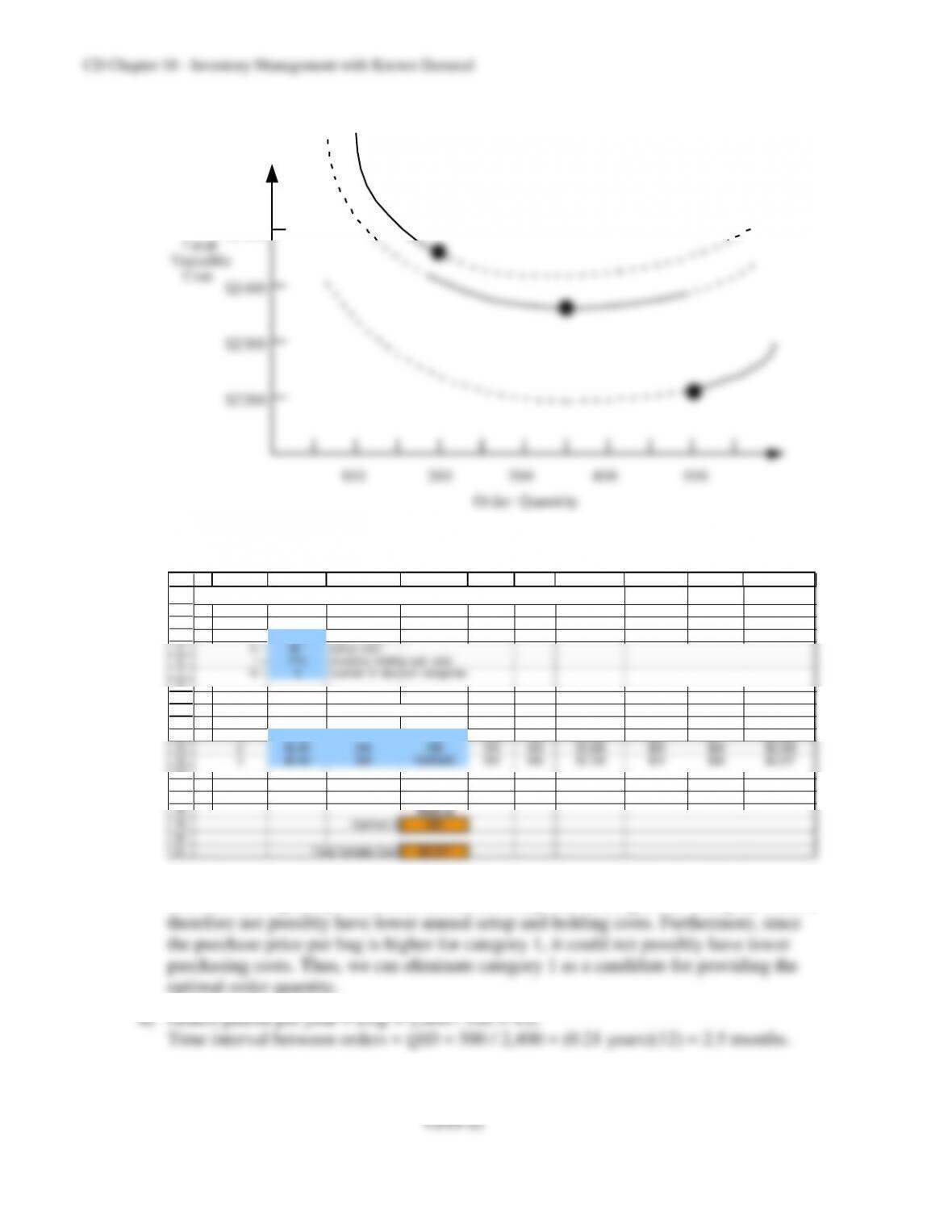
c)
Discount
Category
Feasible
Q
TVC = cD + K(D/Q) = h(Q/2)
1
199
$2,465
2
345
$2,336
3
500
$2,217
1
2
3
4
5
6
7
8
9
10
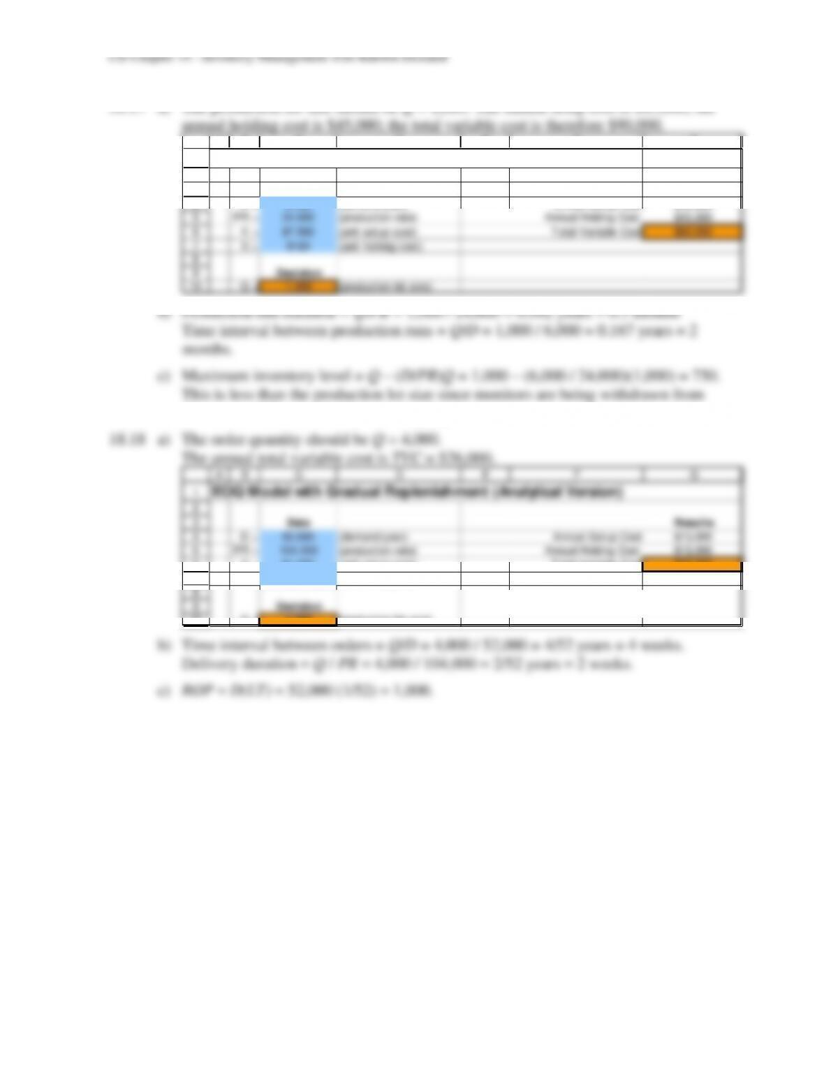
A B C D E F G
EOQ Model with Gradual Replenishment (Analytical Version)
Data Results
D = 6,000 (demand/year) Annual Setup Cost $45,000
PR = 24,000 (production rate) Annual Holding Cost $45,000
K = $7,500 (unit setup cost) Total Variable Cost $90,000
h = $120 (unit holding cost)
Decision
Q = 1,000 (production lot size)
b) Production run duration = Q/PR = 1,000 / 24,000 = 0.042 years = 0.5 months
Time interval between production runs = Q/D = 1,000 / 6,000 = 0.167 years = 2
months.
c) Maximum inventory level = Q – (D/PR)Q = 1,000 – (6,000 / 24,000)(1,000) = 750.
This is less than the production lot size since monitors are being withdrawn from
inventory while a production run is going on.
CD18-24
1
2
3
4
5
6
7
8
9
10
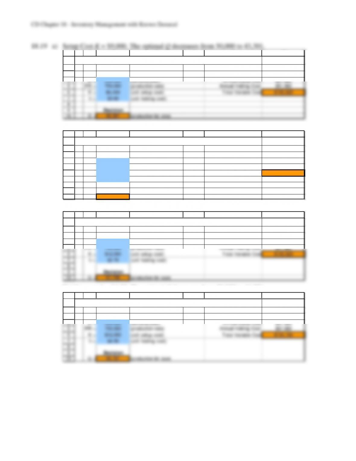
A B C D E F G
EOQ Model with Gradual Replenishment (Analytical Version)
Data Results
D = 250,000 (demand/year) Annual Setup Cost $51,962
PR = 750,000 (production rate) Annual Holding Cost $51,962
K = $9,000 (unit setup cost) Total Variable Cost $103,923
h = $3.60 (unit holding cost)
Decision
Q = 43,301 (production lot size)
Setup Cost K = $15,000. The optimal Q increases from 50,000 to 55,902.
1
2
3
4
5
6
7
8
9
10
A B C D E F G
EOQ Model with Gradual Replenishment (Analytical Version)
Data Results
D = 250,000 (demand/year) Annual Setup Cost $67,082
PR = 750,000 (production rate) Annual Holding Cost $67,082
K = $15,000 (unit setup cost) Total Variable Cost $134,164
h = $3.60 (unit holding cost)
Decision
Q = 55,902 (production lot size)
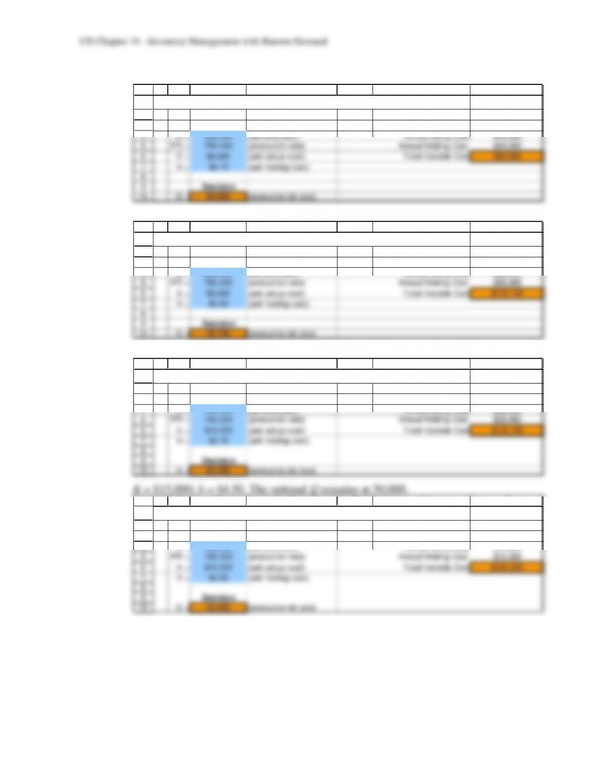
Holding cose h = $2.70. The optimal Q increases from 50,000 to 57,735.
1
2
3
4
5
6
7
8
9
10
A B C D E F G
EOQ Model with Gradual Replenishment (Analytical Version)
Data Results
D = 250,000 (demand/year) Annual Setup Cost $51,962
PR = 750,000 (production rate) Annual Holding Cost $51,962
K = $12,000 (unit setup cost) Total Variable Cost $103,923
h = $2.70 (unit holding cost)
Decision
Q = 57,735 (production lot size)
Holding cost h = $4.50. The optimal Q decreases from 50,000 to 44,721.
1
2
3
4
5
6
7
8
9
10
A B C D E F G
EOQ Model with Gradual Replenishment (Analytical Version)
Data Results
D = 250,000 (demand/year) Annual Setup Cost $67,082
PR = 750,000 (production rate) Annual Holding Cost $67,082
K = $12,000 (unit setup cost) Total Variable Cost $134,164
h = $4.50 (unit holding cost)
Decision
Q = 44,721 (production lot size)
CD18-25
b) K = $9,000; h = $2.70. The optimal Q remains 50,000.
1
2
3
4
5
6
7
8
9
10
A B C D E F G
EOQ Model with Gradual Replenishment (Analytical Version)
Data Results
D = 250,000 (demand/year) Annual Setup Cost $45,000
PR = 750,000 (production rate) Annual Holding Cost $45,000
K = $9,000 (unit setup cost) Total Variable Cost $90,000
h = $2.70 (unit holding cost)
Decision
Q = 50,000 (production lot size)
K = $9,000; h = $4.50. The optimal Q decreases from 50,000 to 38,730.
1
2
3
4
5
6
7
8
9
10
A B C D E F G
EOQ Model with Gradual Replenishment (Analytical Version)
Data Results
D = 250,000 (demand/year) Annual Setup Cost $58,095
PR = 750,000 (production rate) Annual Holding Cost $58,095
K = $9,000 (unit setup cost) Total Variable Cost $116,190
h = $4.50 (unit holding cost)
Decision
Q = 38,730 (production lot size)
K = $15,000; h = $2.70. The optimal Q increases from 50,000 to 64,550.
1
2
3
4
5
6
7
8
9
10
A B C D E F G
EOQ Model with Gradual Replenishment (Analytical Version)
Data Results
D = 250,000 (demand/year) Annual Setup Cost $58,095
PR = 750,000 (production rate) Annual Holding Cost $58,095
K = $15,000 (unit setup cost) Total Variable Cost $116,190
h = $2.70 (unit holding cost)
Decision
Q = 64,550 (production lot size)
K = $15,000; h = $4.50. The optimal Q remains at 50,000.
1
2
3
4
5
6
7
8
9
10
A B C D E F G
EOQ Model with Gradual Replenishment (Analytical Version)
Data Results
D = 250,000 (demand/year) Annual Setup Cost $75,000
PR = 750,000 (production rate) Annual Holding Cost $75,000
K = $15,000 (unit setup cost) Total Variable Cost $150,000
h = $4.50 (unit holding cost)
Decision
Q = 50,000 (production lot size)
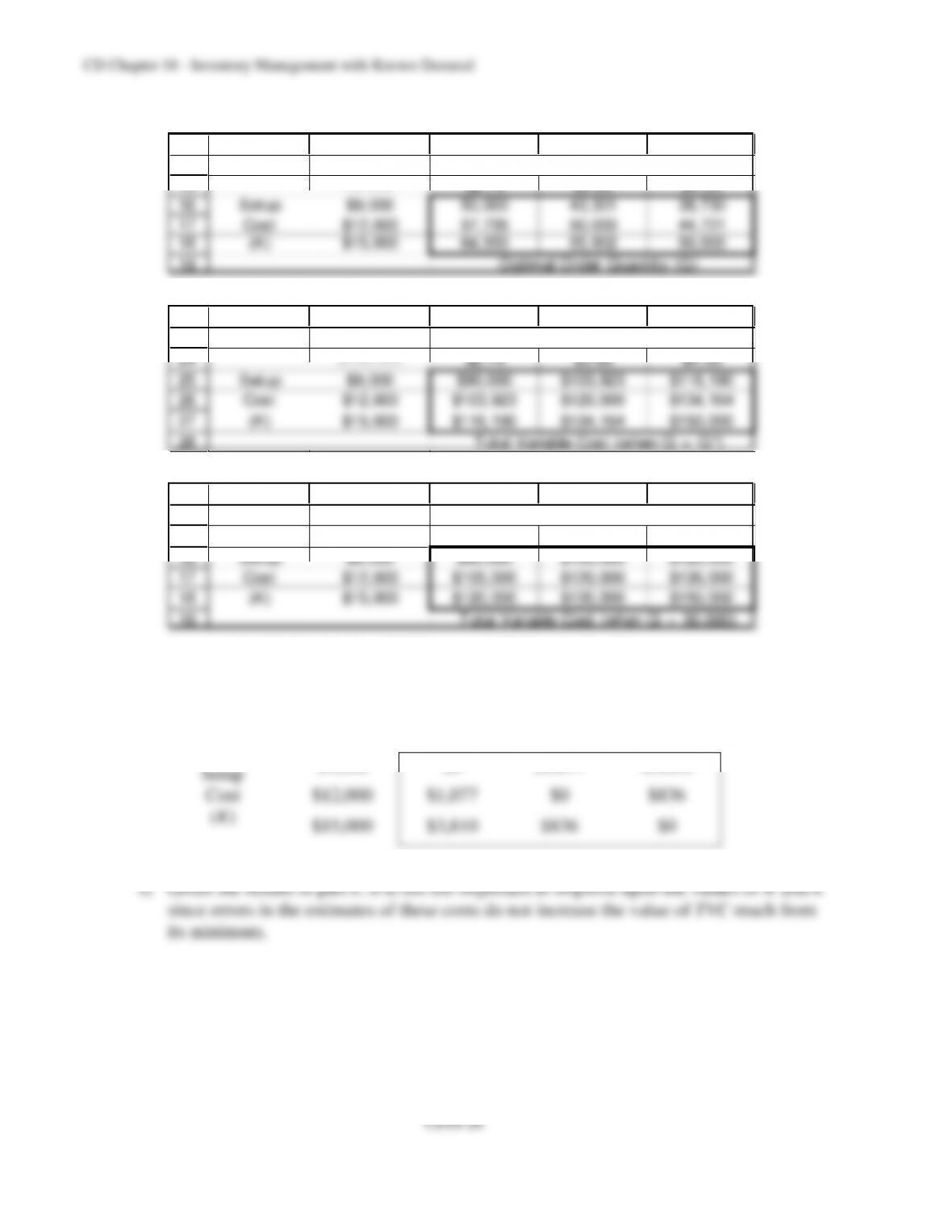
c) The value of Q* is fairly sensitive to the estimates of K and h in all cases except when
both K and h are increased or decreased by the same proportional amount.
CD18-27
18.20 a) This alternative does not look good since it increases TVC by $14,164 to $134,164.
1
2
3
4
5
6
7
8
9
10
A B C D E F G
EOQ Model with Gradual Replenishment (Analytical Version)
Data Results
D = 250,000 (demand/year) Annual Setup Cost $67,082
PR = 1,500,000 (production rate) Annual Holding Cost $67,082
K = $12,000 (unit setup cost) Total Variable Cost $134,164
h = $3.60 (unit holding cost)
Decision
Q = 44,721 (production lot size)
b) There would be only one setup to start the process, and virtually no inventory, so TVC
would be essentially zero.
c) Option 2 is a just-in-time inventory system.
Case
18.1 a) Robert’s problem can be solved using the basic EOQ model. The data for the case is as
follows:
D = 12(250) = 3,000 / year
1
2
3
4
5
6
7
8
9
10
11
A B C D E F G
Basic EOQ Model (Analytical Version)
Data Results
D = 3,000 (demand/year) Reorder Point 0
K = $6.25 (setup cost)
h = $0.15 (unit holding cost) Annual Setup Cost $37.50
L = 0 (lead time in days) Annual Holding Cost $37.50
WD = 360 (working days/year) Total Variable Cost $75.00
Decision
Q = 500 (optimal order quantity)
CD18-28
b) Now the lead time is L = 5 days. We can use the basic EOQ model again:
1
2
3
4
5
6
7
8
9
10
11
A B C D E F G
Basic EOQ Model (Analytical Version)
Data Results
D = 3,000 (demand/year) Reorder Point 41.7
K = $6.25 (setup cost)
h = $0.15 (unit holding cost) Annual Setup Cost $37.50
L = 5 (lead time in days) Annual Holding Cost $37.50
WD = 360 (working days/year) Total Variable Cost $75.00
Decision
Q = 500 (optimal order quantity)
Whenever the inventory of toothbrushes drops below 42, Robert should place an order
for 500 toothbrushes. He needs to place an order 6 times a year.
1
2
3
4
5
6
7
8
9
10
11
A B C D E F G
EOQ Model with Planned Shortages (Analytical Version)
Data Results
D = 3,000 (demand/year) Max Inventory Level 483.8
K = $6.25 (setup cost)
h = $0.15 (unit holding cost) Annual Setup Cost $36.28
p = $2.20 (unit shortage cost) Annual Holding Cost $33.97
Annual Shortage Cost $2.32
Decision Total Variable Cost $72.57
Q = 517 (optimal order quantity)
S = 33 (optimal maximum shortage)
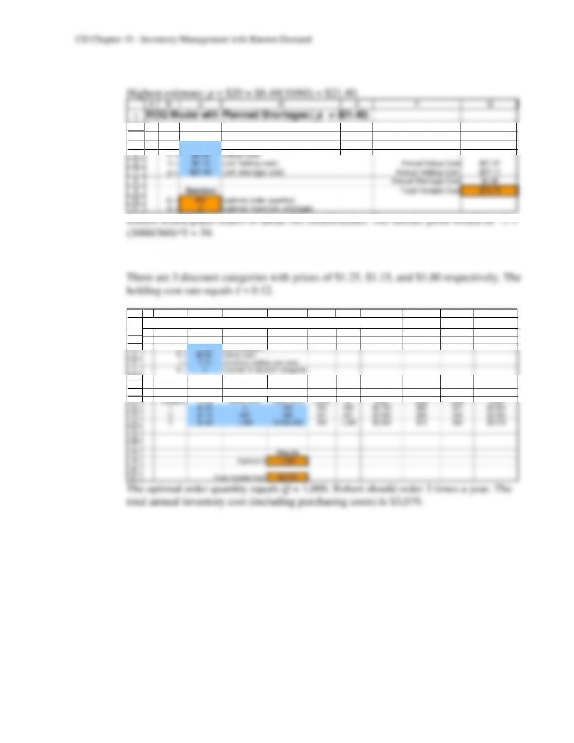
would be roughly 33 toothbrushes.
d) We compute the inventory policies for the two extreme cases.
Lowest estimate: p = $0 + $8.40(3/60) = $0.42:
1
2
3
4
5
6
7
8
9
10
11
A B C D E F G
EOQ Model with Planned Shortages ( p = $0.42)
Data Results
D = 3,000 (demand/year) Max Inventory Level 429.2
K = $6.25 (setup cost)
h = $0.15 (unit holding cost) Annual Setup Cost $32.19
p = $0.42 (unit shortage cost) Annual Holding Cost $23.72
Annual Shortage Cost $8.47
Decision Total Variable Cost $64.38
Q = 582 (optimal order quantity)
S = 153 (optimal maximum shortage)
Robert would place orders of about 582 toothbrushes. The reorder point would be –153
+ (3000/360)*5 = –111.