CD18-1
CD Chapter 18 Inventory Management with Known Demand
Review Questions
18.1-1 Administrative costs, such as labor charges to place an order, can cause the cost to exceed
the purchase price.
18.1-2 Capital tied up in inventory will not be regained until the goods are sold. If the capital
were free to be invested it would be able to earn a return from other opportunities. This
18.1-3 Other costs associated with holding inventory include the cost of leasing warehouse space,
the cost of insurance for inventory, labor costs for warehouse personnel, and taxes based
18.1-4 Customer dissatisfaction and the loss of future sales, price decreases to compensate for
18.2-1 The four cost components that may be included in an inventory model are acquisition cost,
setup cost, holding cost, and shortage cost.
18.2-3 When the replenishment is done by purchasing the product, the setup cost consists of the
various administrative costs. When a manufacturer is replenishing its inventory, the setup
cost consists of the cost of setting up the manufacturing process for another production
run.
18.2-4 An inventory policy prescribes both when inventory should be replenished and by how
much.
18.2-5 The total inventory cost per unit time needs to be minimized to determine an optimal
inventory policy.
18.2-6 A fixed cost is a cost that remains the same regardless of the decisions made while a
18.3-1 The basic EOQ model is so popular due to a combination of simplicity and wide
applicability.

CD Chapter 18 – Inventory Management with Known Demand
CD18-2
18.3-2 The model assumes a constant demand rate, that the order quantity to replenish inventory
CD18-3
18.3-3 Lead-time is the amount of time between the placement of an order and the delivery of the
order quantity. The reorder point is the inventory level at which an order is placed.
18.3-5 A continuous-review inventory system will not fit the basic EOQ model if shortages often
occur and it is necessary to carry safety stock.
18.4-1 The two types of costs included in the total variable cost are the annual setup cost and the
18.4-2 The optimal order quantity increases if the demand rate increases in order to avoid overly
large increases in the number of setup costs incurred per year. The optimal order quantity
18.4-3 The optimal order quantity can change fairly significantly if fairly small changes are made
to either the setup cost of the unit holding cost. This change is even larger if the changes
are made to both costs in opposite directions.
18.4-4 The optimal order quantity does not change if both the setup cost and the unit holding cost
are changed by the same percentage amount in the same direction.
costs.
18.5-1 If the cost of holding inventory is high relative to the shortage costs then it may make
sense to permit planned inventory shortages.
18.5-3 The decision variables for the EOQ model with planned shortages are the order quantity Q
and the maximum shortage S.
18.5-5 The optimal order quantity for this model is larger than for the basic EOQ model. The
maximum inventory level for this model always will be less than for the basic EOQ
model.

CD18-4
18.6-1 Quantity discounts are reductions in the unit acquisition costs of a product that are offered
for ordering a relatively large quantity.
CD18-5
18.6-2 When quantity discounts are offered, annual acquisition costs need to be included in the
total variable inventory cost.
18.6-3 The unit holding cost is equal to the price paid for the items in inventory multiplied by the
inventory holding cost rate (h = Ic).
18.6-4 The best order quantity for a discount category whose minimum order quantity exceeds Q
18.7-1 The replenishment of inventory over time is common with manufacturers who replenish
their inventory by conducting intermittent production runs.
18.7-2 The assumptions for this model are the same as those for the basic EOQ model except that
a production run is scheduled to begin each time the inventory level drops to 0, and this
production run replenishes inventory at a constant rate throughout the duration of the run.
18.7-3 The maximum inventory level is less than the production lot size because products are
being withdrawn from inventory as the production run is under way.
18.7-5 Independent-demand products have demand that does not depend on the demands for all
18.7-6 Material requirements planning (MRP) is a popular technique for managing inventories of
components of a final product.
18.7-8 In more general terms, the focus of the just-in-time philosophy is on avoiding waste
wherever it might occur in the production process.
CD18-6
Problems
18.1 a)
1
2
3
4
5
6
7
8
9
10
11
A B C D E F G
Basic EOQ Model (Solver Version)
Data Results
D = 676 (demand/year) Reorder Point 6.5
K = $75 (setup cost)
h = $600 (unit holding cost) Annual Setup Cost $10,140
L = 3.5 (lead time in days) Annual Holding Cost $1,500
WD = 365 (working days/year) Total Variable Cost $11,640
Decision
Q = 5
b)
14
15
16
17
18
19
20
21
22
23
24
25
26
27
28
C D E F
Annual Annual Total
Setup Holding Variable
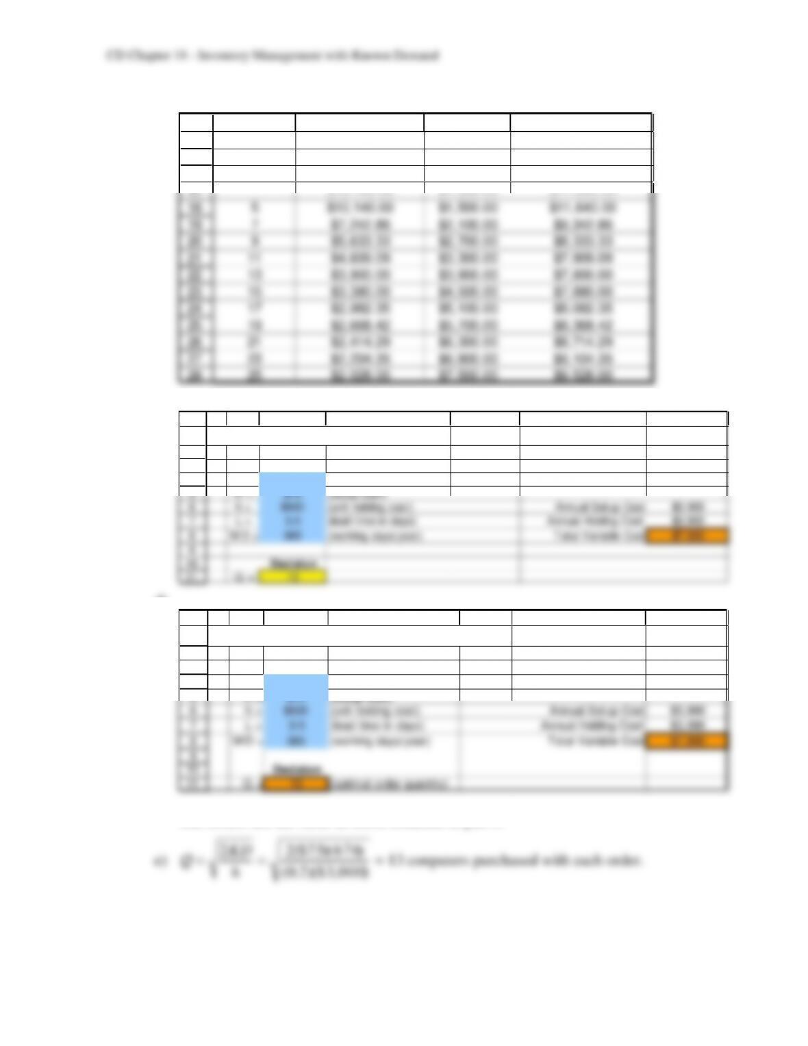
Q Cost Cost Cost
$10,140.00 $1,500.00 $11,640.00
5 $10,140.00 $1,500.00 $11,640.00
7 $7,242.86 $2,100.00 $9,342.86
9 $5,633.33 $2,700.00 $8,333.33
11 $4,609.09 $3,300.00 $7,909.09
13 $3,900.00 $3,900.00 $7,800.00
15 $3,380.00 $4,500.00 $7,880.00
17 $2,982.35 $5,100.00 $8,082.35
19 $2,668.42 $5,700.00 $8,368.42
21 $2,414.29 $6,300.00 $8,714.29
23 $2,204.35 $6,900.00 $9,104.35
25 $2,028.00 $7,500.00 $9,528.00
c)
1
2
3
4
5
6
7
8
9
10
11
A B C D E F G
Basic EOQ Model (Solver Version)
Data Results
D = 676 (demand/year) Reorder Point 6.5
K = $75 (setup cost)
h = $600 (unit holding cost) Annual Setup Cost $3,900
L = 3.5 (lead time in days) Annual Holding Cost $3,900
WD = 365 (working days/year) Total Variable Cost $7,800
Decision
Q = 13
d)
1
2
3
4
5
6
7
8
9
10
11
A B C D E F G
Basic EOQ Model (Analytical Version)
Data Resu lts
D = 676 (demand/year) Reorder Point 6.5
K = $75 (setup cost)
h = $600 (unit holding cost) Annual Setup Cost $3,900
L = 3.5 (lead time in days) Annual Holding Cost $3,900
WD = 365 (working days/year) Total Variable Cost $7,800
Decision
Q = 13 (optimal order quantity)
The results are the same as those obtained in part c.
CD18-8
18.2 a)
1
2
3
4
5
6
7
8
9
10
11
A B C D E F G
Basic EOQ Model (Solver Version)
Data Results
D = 102,000 (demand/year) Reorder Point 0
K = $1,000 (setup cost)
h = $0.12 (unit holding cost) Annual Setup Cost $12,000
L = 0 (lead time in days) Annual Holding Cost $510
WD = 365 (working days/year) Total Variable Cost $12,510
Decision
Q = 8,500
b)
14
15
16
17
18
19
20
21
22
23
24
25
26
27
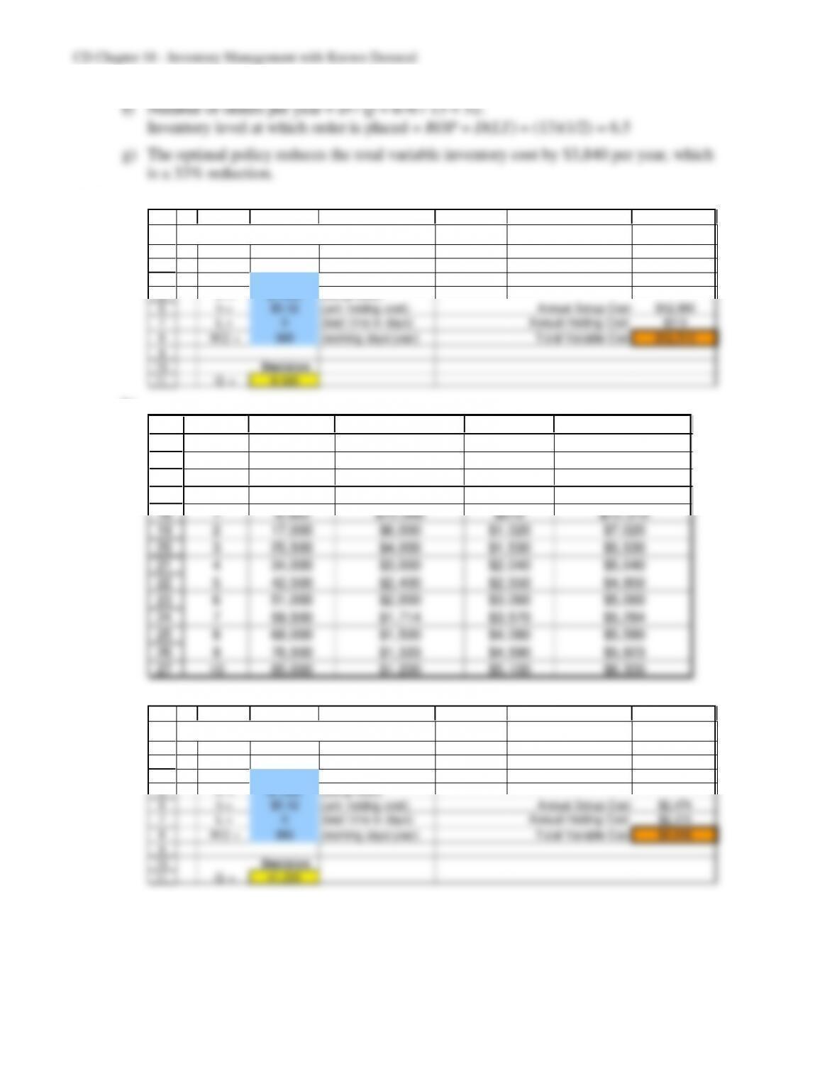
B C D E F
Annual Annual Total
Setup Holding Variable
Months Q Cost Cost Cost
$12,000 $510 $12,510
1 8,500 $12,000 $510 $12,510
2 17,000 $6,000 $1,020 $7,020
3 25,500 $4,000 $1,530 $5,530
4 34,000 $3,000 $2,040 $5,040
5 42,500 $2,400 $2,550 $4,950
6 51,000 $2,000 $3,060 $5,060
7 59,500 $1,714 $3,570 $5,284
8 68,000 $1,500 $4,080 $5,580
9 76,500 $1,333 $4,590 $5,923
10 85,000 $1,200 $5,100 $6,300
c)
1
2
3
4
5
6
7
8
9
10
11
A B C D E F G
Basic EOQ Model (Solver Version)
Data Results
D = 102,000 (demand/year) Reorder Point 0
K = $1,000 (setup cost)
h = $0.12 (unit holding cost) Annual Setup Cost $2,474
L = 0 (lead time in days) Annual Holding Cost $2,474
WD = 365 (working days/year) Total Variable Cost $4,948
Decision
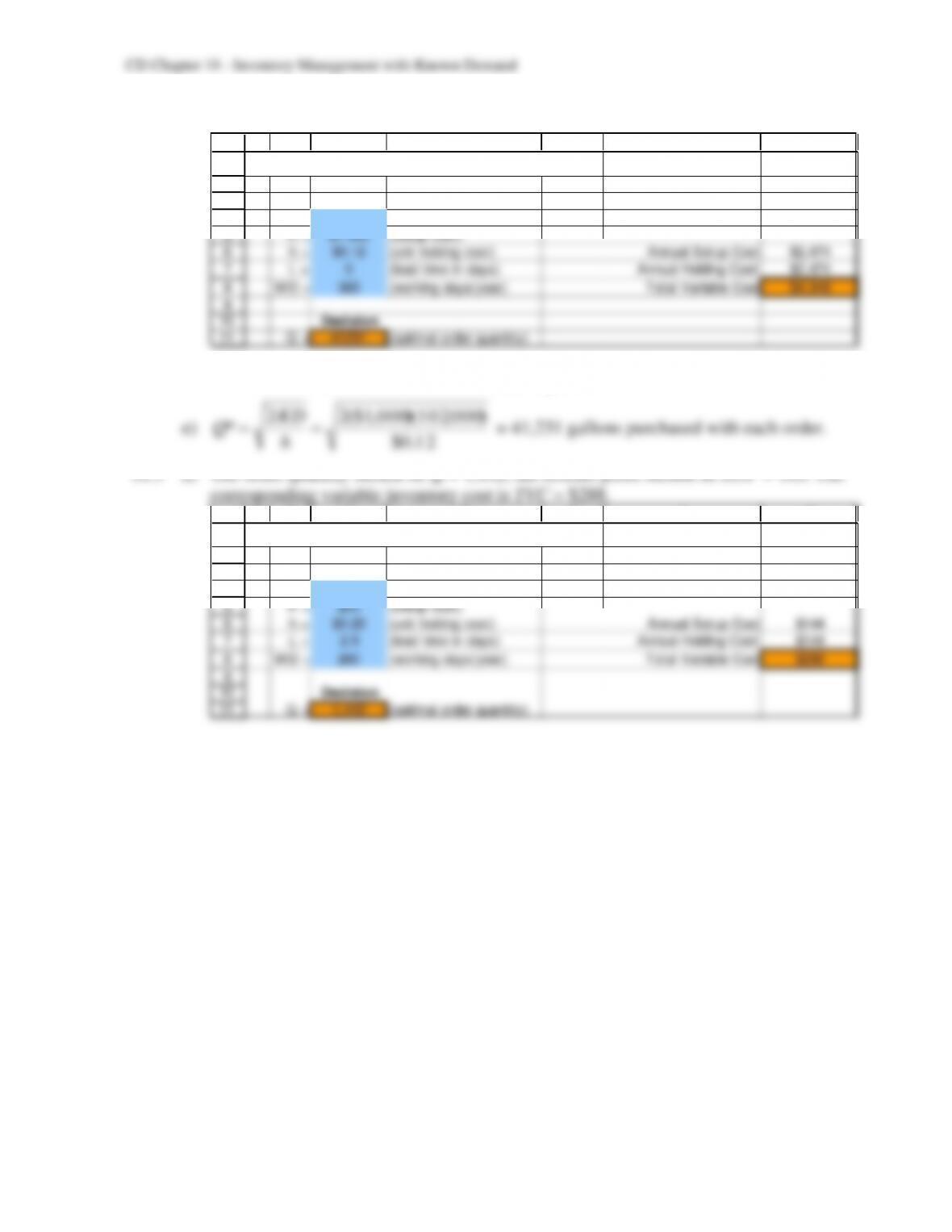
Q = 41,231
1
2
3
4
5
6
7
8
9
10
11
A B C D E F G
Basic EOQ Model (Analytical Version)
Data Resu lts
D = 10,400 (demand/year) Reorder Point 100
K = $20 (setup cost)
h = $0.20 (unit holding cost) Annual Setup Cost $144
L = 2.5 (lead time in days) Annual Holding Cost $144
WD = 260 (working days/year) Total Variable Cost $288
Decision
Q = 1,442 (optimal order quantity)
d)
1
2
3
4
5
6
7
8
9
10
11
A B C D E F G
Basic EOQ Model (Analytical Version)
Data Resu lts
D = 102,000 (demand/year) Reorder Point 0
K = $1,000 (setup cost)
h = $0.12 (unit holding cost) Annual Setup Cost $2,474
L = 0 (lead time in days) Annual Holding Cost $2,474
WD = 365 (working days/year) Total Variable Cost $4,948
Decision
Q = 41231 (optimal order quantity)
The results are the same as those obtained in part c.
CD18-10
b) The new order quantity should be Q = 1,665 with TVC = $250. The order quantity is
increased by 223 LCDs.
1
2
3
4
5
6
7
8
9
10
11
A B C D E F G
Basic EOQ Model (Analytical Version)
Data Resu lts
D = 10,400 (demand/year) Reorder Point 100
K = $20 (setup cost)
h = $0.15 (unit holding cost) Annual Setup Cost $125
L = 2.5 (lead time in days) Annual Holding Cost $125
WD = 260 (working days/year) Total Variable Cost $250
Decision
Q = 1,665 (optimal order quantity)
If the order quantity obtained in part a is still used the TVC increases to $252.
1
2
3
4
5
6
7
8
9
10
11
A B C D E F G
Basic EOQ Model (Solver Version)
Data Results
D = 10,400 (demand/year) Reorder Point 100
K = $20 (setup cost)
h = $0.15 (unit holding cost) Annual Setup Cost $144
L = 2.5 (lead time in days) Annual Holding Cost $108
WD = 260 (working days/year) Total Variable Cost $252
Decision
Q = 1,442
CD18-11
c) The new order quantity should be Q = 1,290 with TVC = $322. The order quantity is
decreased by 152 LCDs.
1
2
3
4
5
6
7
8
9
10
11
A B C D E F G
Basic EOQ Model (Analytical Version)
Data Resu lts
D = 10,400 (demand/year) Reorder Point 100
K = $20 (setup cost)
h = $0.25 (unit holding cost) Annual Setup Cost $161
L = 2.5 (lead time in days) Annual Holding Cost $161
WD = 260 (working days/year) Total Variable Cost $322
Decision
Q = 1,290 (optimal order quantity)
If the order quantity obtained in part a is still used the TVC increases to $324.
1
2
3
4
5
6
7
8
9
10
11
A B C D E F G
Basic EOQ Model (Solver Version)
Data Results
D = 10,400 (demand/year) Reorder Point 100
K = $20 (setup cost)
h = $0.25 (unit holding cost) Annual Setup Cost $144
L = 2.5 (lead time in days) Annual Holding Cost $180
WD = 260 (working days/year) Total Variable Cost $324
Decision
Q = 1,442
d)
15
16
17
18
19
20
21
22
23
24
B C D
Cost Unit Optimal
of Holding Order
Capital Cost Quantity
1,442
10% $0.15 1,665
12% $0.17 1,564
14% $0.19 1,480
16% $0.21 1,407
18% $0.23 1,345
20% $0.25 1,290
CD18-12
e)
15
16
17
18
19
20
21
22
23
B C D
Hours Optimal
of Clerical Setup Order
Time Cost Quantity
1,442
0.5 $10 1,020
0.75 $15 1,249
1$20 1,442
1.25 $25 1,612
1.5 $30 1,766
f)
15
16
17
18
19
20
21
22
23
24
B C D E F G H I
Cost Unit Optimal Order Quantity (Q)
of Holding
Capital Cost 0.5 0.75 1 1.25 1.5 Clerical Hours
1442 $10 $15 $20 $25 $30 Setup Cost
10% $0.15 1,178 1,442 1,665 1,862 2,040
12% $0.17 1,106 1,355 1,564 1,749 1,916
14% $0.19 1,046 1,281 1,480 1,654 1,812
16% $0.21 995 1,219 1,407 1,574 1,724
18% $0.23 951 1,165 1,345 1,504 1,647
20% $0.25 912 1,117 1,290 1,442 1,580
18.4 Optimal Order Quantity:
15
16
17
18
19
20
21
22
23
24
B C D E F G H I J
Unit Holding Cost
573 $3.15 $3.36 $3.78 $4.20 $4.62 $5.04 $5.25
$86.25 573 555 523 496 473 453 444
$92.00 592 573 540 513 489 468 459
Setup $103.50 628 608 573 544 518 496 486
Cost $115.00 662 641 604 573 547 523 513
$126.50 694 672 634 601 573 549 538
$138.00 725 702 662 628 599 573 562
$143.75 740 717 676 641 611 585 573
Optimal Order Quantity
Total Variable Cost (with Q = Q*):
27
28
29
30
31
32
33
34
35
36
B C D E F G H I J
Unit Holding Cost
$2,407 $3.15 $3.36 $3.78 $4.20 $4.62 $5.04 $5.25
$86.25 $1,806 $1,865 $1,978 $2,085 $2,187 $2,284 $2,331
$92.00 $1,865 $1,926 $2,043 $2,153 $2,258 $2,359 $2,407
Setup $103.50 $1,978 $2,043 $2,167 $2,284 $2,395 $2,502 $2,554
Cost $115.00 $2,085 $2,153 $2,284 $2,407 $2,525 $2,637 $2,692
$126.50 $2,187 $2,258 $2,395 $2,525 $2,648 $2,766 $2,823
$138.00 $2,284 $2,359 $2,502 $2,637 $2,766 $2,889 $2,949
$143.75 $2,331 $2,407 $2,554 $2,692 $2,823 $2,949 $3,009
Total Variable Cost (with Q = Q*)
Total Variable Cost (with Q = 573):
17
18
19
20
21
22
23
24
25
26
B C D E F G H I J
Unit Holding Cost
$2,407 $3.15 $3.36 $3.78 $4.20 $4.62 $5.04 $5.25
$86.25 $1,806 $1,866 $1,986 $2,106 $2,227 $2,347 $2,407
$92.00 $1,866 $1,926 $2,046 $2,167 $2,287 $2,407 $2,467
Setup $103.50 $1,986 $2,046 $2,167 $2,287 $2,407 $2,528 $2,588
Cost $115.00 $2,107 $2,167 $2,287 $2,407 $2,528 $2,648 $2,708
$126.50 $2,227 $2,287 $2,408 $2,528 $2,648 $2,769 $2,829
$138.00 $2,348 $2,408 $2,528 $2,648 $2,769 $2,889 $2,949
$143.75 $2,408 $2,468 $2,588 $2,709 $2,829 $2,949 $3,009
Total Variable Cost (with Q = 573)
The conclusions remain basically the same when the estimates could be off by as much as
25%. In the cases where K and h change in the same direction, there is little or no extra
18.5 a) Q* will decrease by half.
b) Q* will double.
CD18-14
b) The optimal order quantity when h = (20%)($20) = $4 is 150. The annual TVC = $600.
1
2
3
4
5
6
7
8
9
10
11
A B C D E F G
Basic EOQ Model (Analytical Version)
Data Resu lts
D = 600 (demand/year) Reorder Point 10
K = $75 (setup cost)
h = $4 (unit holding cost) Annual Setup Cost $300
L = 5 (lead time in days) Annual Holding Cost $300
WD = 300 (working days/year) Total Variable Cost $600
Decision
Q = 150 (optimal order quantity)
With the current inventory policy (Q = 50), the annual TVC = $1,000.
1
2
3
4
5
6
7
8
9
10
11
A B C D E F G
Basic EOQ Model
Data Results
D = 600 (demand/year) Reorder Point 10
K = $75 (setup cost)
h = $4 (unit holding cost) Annual Setup Cost $900
L = 5 (lead time in days) Annual Holding Cost $100
WD = 300 (working days/year) Total Variable Cost $1,000
Decision
Q = 50
c) Reorder point is 10 as shown in the above spreadsheet.
h 10=2($200)D
$400 D=10
2($200)
18.8 TVC = K(D/Q) + h(Q/2)
TVC
Q
= −KD
Q2+h
2=0 KD
Q2=2KD
h Q=2KD
h.
18.9 a) The optimal order quantity is Q = 245 with annual TVC = $4,899.
1
2
3
4
5
6
7
8
9
10
11
A B C D E F G
Basic EOQ Model (Analytical Version)
Data Resu lts
D = 3,000 (demand/year) Reorder Point 0
K = $200 (setup cost)
h = $20 (unit holding cost) Annual Setup Cost $2,449
L = 0 (lead time in days) Annual Holding Cost $2,449
WD = 300 (working days/year) Total Variable Cost $4,899
Decision
Q = 245 (optimal order quantity)
CD18-15
b) The new optimal order quantity is Q = 316, with a maximum shortage of S = 126.
1
2
3
4
5
6
7
8
9
10
11
A B C D E F G
EOQ Model with Planned Shortages (Analytical Version)
Data Results
D = 3,000 (demand/year) Max Inventory Level 190
K = $200 (setup cost)
h = $20 (unit holding cost) Annual Setup Cost $1,897
p = $30 (unit shortage cost) Annual Holding Cost $1,138
Annual Shortage Cost $759
Decision Total Variable Cost $3,795
Q = 316 (optimal order quantity)
S = 126 (optimal maximum shortage)
c)
Quantity
Basic EOQ
Model
EOQ Model with
Planned Shortages
Order quantity
245
316
Maximum shortage
0
126
Maximum inventory level
245
190
Reorder point
0
-126
Annual setup cost
$2,449
$1,897
Annual holding cost
$2,449
$1,138
Annual shortage cost
$0
$759
Total variable cost
$4,899
$3,795