CD15-1
CD Chapter 15 Transportation and Assignment Problems
Review Questions
15.1-1 The CEO is concerned about escalating costs, in particular the shipping costs for peas.
15.1-2 Kim Baker is being asked to look at the current shipping plan and see if they can develop a
new one that would reduce the total shipping cost to an absolute minimum.
15.2-2 The data needed for a transportation problem are the supplies, demands, and unit costs.
15.2-3 Formulating a problem as a transportation problem only requires filling out a table in the
format of Table 15.5.
15.2-5 As long as all its supplies and demands have integer values, any transportation problem
with feasible solutions is guaranteed to have an optimal solution with integer values for all
its decision variables.
15.3-2 Instead of a demand row, there is both a minimum row and a maximum row. Then
constraints are entered so that Shipped ≥ Minimum and Shipped ≤ Maximum.
15.4-2 Minimize the total cost of meeting the water needs of the four cities they serve.
15.4-3 The sources are the production of jet engines on regular time and overtime in each of the
four months. The destinations are their installation in each of the four months.
15.5-1 The three key factors are (1) the cost of transporting the oil from its sources to all the
15.5-2 The new refinery will have a great impact on the operation of the entire distribution system,
including decisions on how much to ship to and from each refinery (new and old).
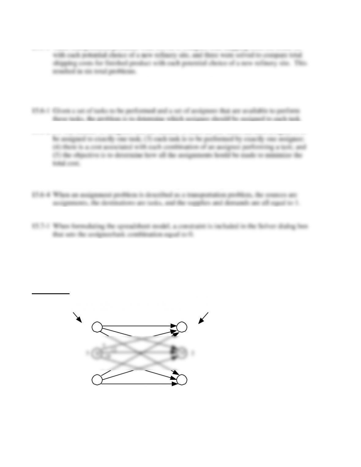
15.5-3 Three transportation problems were solved to compare total shipping costs for crude oil
15.5-4 Management must consider non-financial factors as well, such as closeness to corporate
headquarters and whether there are any cost trends or trends in the marketplace that might
alter the picture in the future.
15.6-2 (1) The number of assignees and the number of tasks are the same; (2) each assignee is to
15.6-3 (1) Identify the assignees and tasks, and (2) construct a cost table that gives the cost
associated with each combination of an assignee performing a task.
15.6-5 The Hungarian method solves assignment problems well.
15.7-2 If an assignee will perform more than one task, the supply is change from 1 to the greater
amount that can be performed.
15.7-3 If a task will be performed by more than one assignee, the demand is changed from 1 to the
greater amount.
Problems
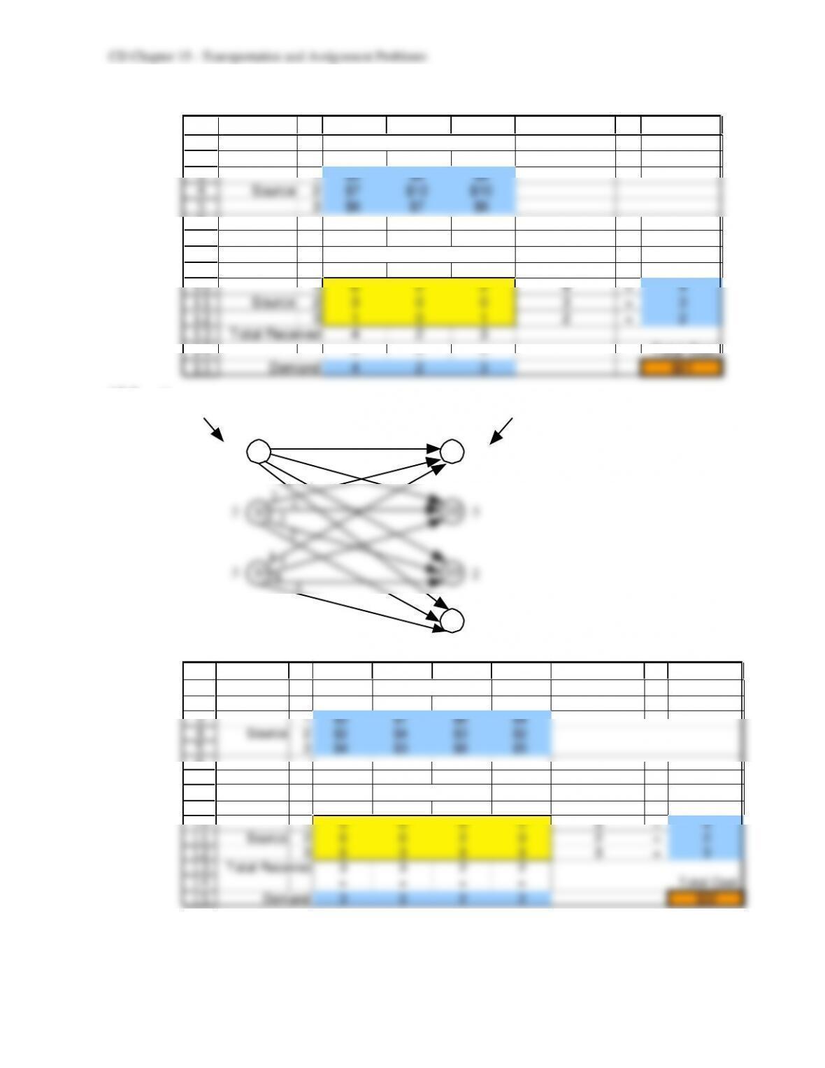
15.1 a)
S1
D2
S2
S3
D1
D3
So urces De st in at io ns
9
6
8
712
10
67
6
4
3
2
4
2
3
Su ppl i es De ma nds
b)
1
2
3
4
5
6
7
8
9
10
11
12
13
14
15
A B C D E F G H
Unit Cost Destination
1 2 3
1$9 $6 $8
Source 2 $7 $12 $10
3$6 $7 $6
Shipments Destination
1 2 3 Total Shipped Supply
1 0 2 2 4 = 4
Source 2 3 0 0 3 = 3
3 1 0 1 2 = 2
Total Received 4 2 3
= = = Total Cost
Demand 4 2 3 $61
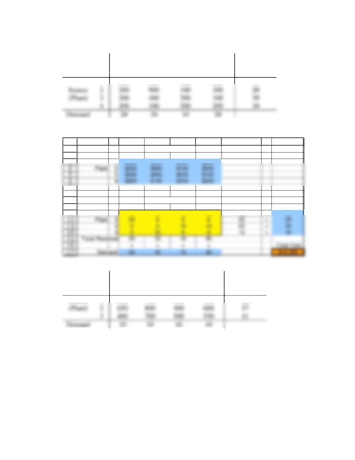
15.2 a)
S1
D2
S2
S3
D1
D3
So urces De st in at io ns
3
7
6
24
3
43
8
5
2
3
3
3
2
Su ppl i es De ma nds
D4 2
4
2
5
b)
1
2
3
4
5
6
7
8
9
10
11
12
13
14
15
A B C D E F G H I
Unit Cost
1 2 3 4
1$3 $7 $6 $4
Source 2 $2 $4 $3 $2
3$4 $3 $8 $5
Shipments
1 2 3 4 Total Shipped Supply
1 3 0 0 2 5 = 5
Source 2 0 0 2 0 2 = 2
3 0 3 0 0 3 = 3
Total Received 3 3 2 2
= = = = Total Cost
Demand 3 3 2 2 $32
Destination
Destination
CD15-4
15.3 a)
Unit Cost ($)
Destination (Retail Outlet)
1
2
3
4
Supply
1
500
600
400
200
10
Source
2
200
900
100
300
20
(Plant)
3
300
400
200
100
20
4
200
100
300
200
10
Demand
20
10
10
20
b)
1
2
3
4
5
6
7
8
9
10
11
12
13
14
15
16
17
A B C D E F G H I
Unit Cost
1 2 3 4
1 $500 $600 $400 $200
Plant 2 $200 $900 $100 $300
3 $300 $400 $200 $100
4 $200 $100 $300 $200
Shipments
1 2 3 4 Total Shipped Supply
1 0 0 0 10 10 =10
Plant 2 20 0 0 0 20 =20
3 0 0 10 10 20 =20
4 0 10 0 0 10 =10
Total Received 20 10 10 20
= = = = Total Cost
Demand 20 10 10 20 $10,000
Retail Outlet
Retail Outlet
15.4 a)
Unit Cost ($)
Destination (Distribution Center)
1
2
3
4
Supply
Source
1
500
750
300
450
12
(Plant)
2
650
800
400
600
17
3
400
700
500
550
11
Demand
10
10
10
10
CD15-5
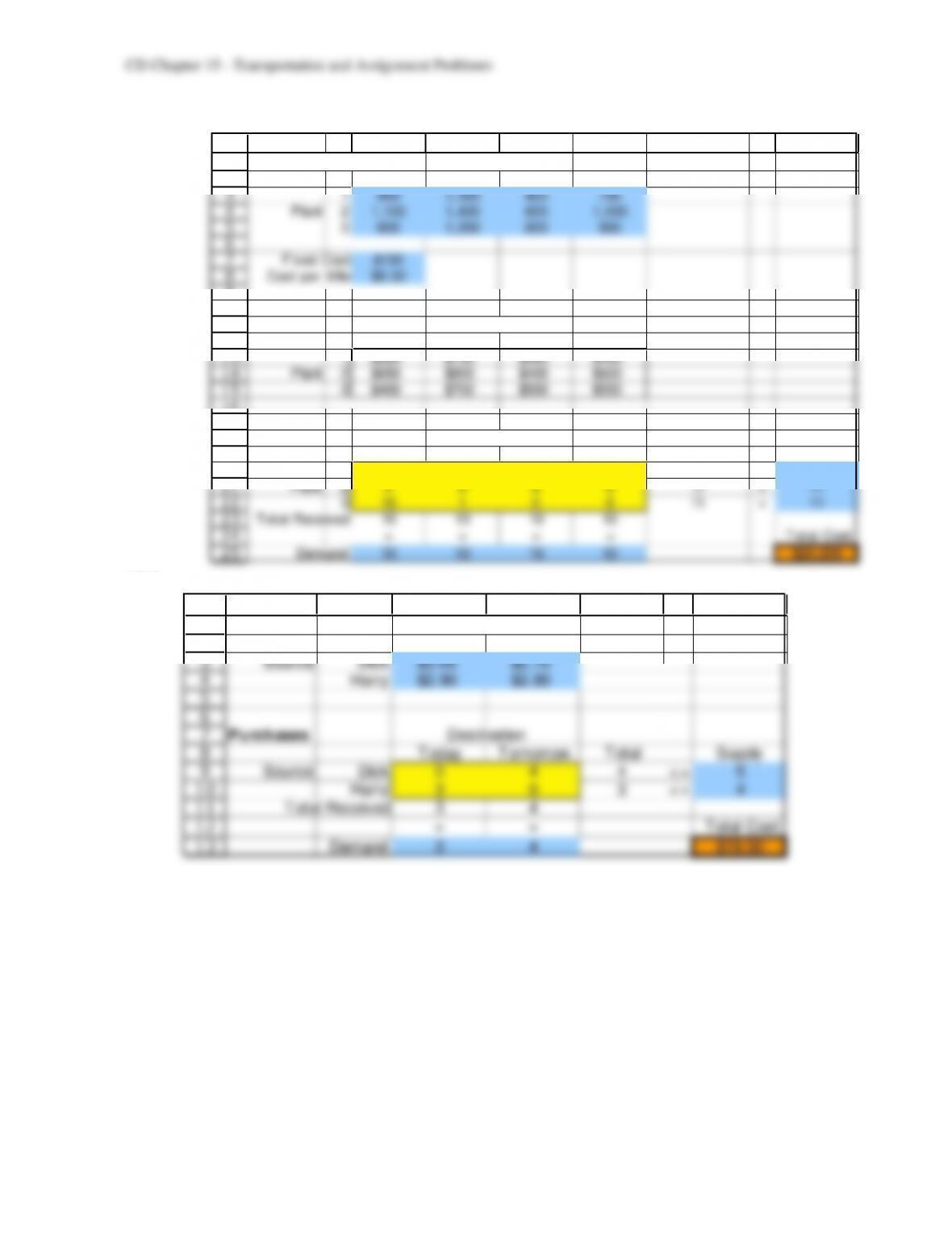
b)
1
2
3
4
5
6
7
8
9
10
11
12
13
14
15
16
17
18
19
20
21
22
23
24
25
A B C D E F G H I
Distance (miles)
1 2 3 4
1 800 1,300 400 700
Plant 2 1,100 1,400 600 1,000
3 600 1,200 800 900
Fixed Cost $100
Cost per Mile $0.50
Unit Cost
1 2 3 4
1 $500 $750 $300 $450
Plant 2 $650 $800 $400 $600
3 $400 $700 $500 $550
Shipments
1 2 3 4 Total Shipped Supply
1 0 0 2 10 12 =12
Plant 2 0 9 8 0 17 =17
310 1 0 0 11 =11
Total Received 10 10 10 10
= = = = Total Cost
Demand 10 10 10 10 $20,200
Distribution Center
Distribution Center
Distribution Center
15.5
1
2
3
4
5
6
7
8
9
10
11
12
13
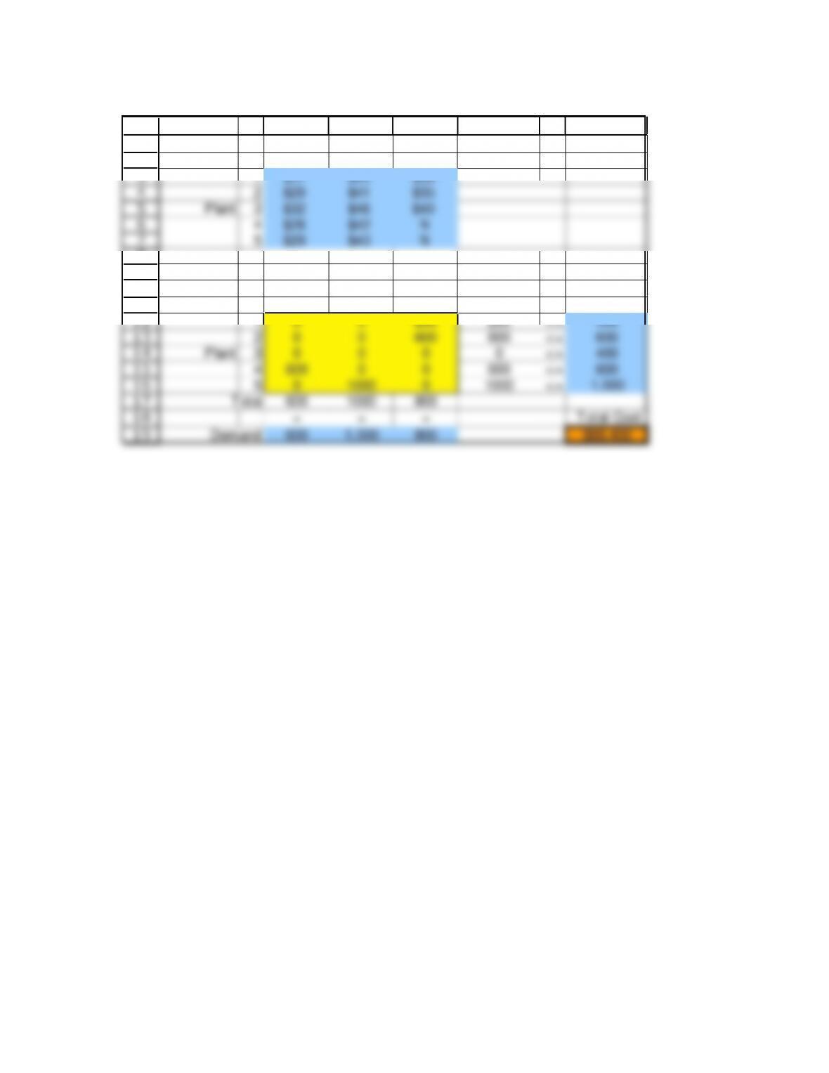
A B C D E F G
Unit Cost
Today Tomorrow
Source Dick $3.00 $2.70
Harry $2.90 $2.80
Purchases
Today Tomorrow Total Supply
Source Dick 0 4 4 <= 5
Harry 3 0 3 <= 4
Total Received 3 4
= = Total Cost
Demand 3 4 $19.50
Destination
Destination
CD15-6
15.6
1
2
3
4
5
6
7
8
9
10
11
12
13
14
15
16
17
18
19
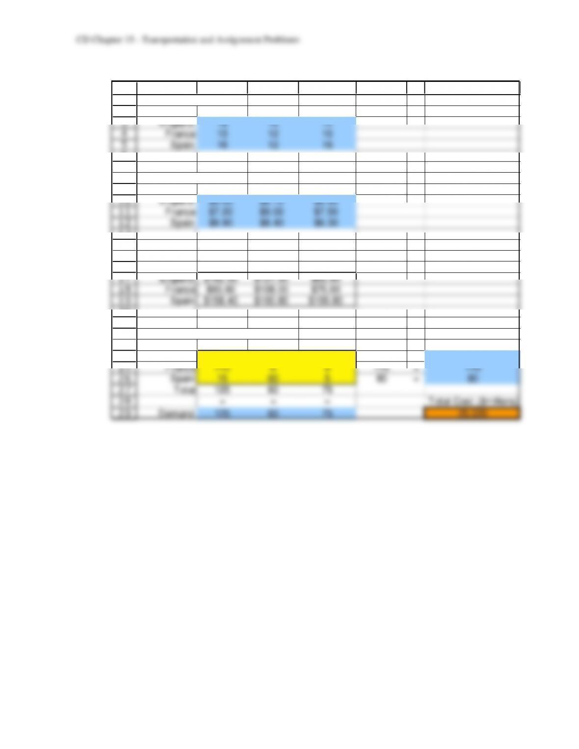
A B C D E F G H
Unit Cost Product
1 2 3
1 $31 $45 $38
2 $29 $41 $35
Plant 3 $32 $46 $40
4 $28 $42 Ń
5 $29 $43 Ń
Production Product
1 2 3 Total Supply
1 0 0 200 200 <= 400
2 0 0 600 600 <= 600
Plant 3 0 0 0 0 <= 400
4 600 0 0 600 <= 600
5 0 1000 0 1000 <= 1,000
Total 600 1000 800
= = = Total Cost
Demand 600 1,000 800 $88,400
CD15-7
15.7
1
2
3
4
5
6
7
8
9
10
11
12
13
14
15
16
17
18
19
20
21
22
23
24
25
26
27
28
29
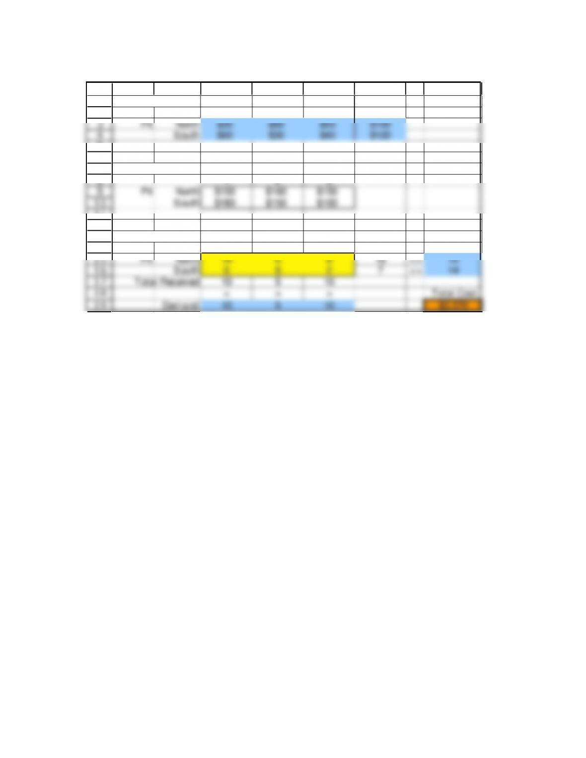
A B C D E F G
Labor Hours / Acre
W heat Barley O ats
England 18 15 12
France 13 12 10
Spain 16 12 16
Labor Cost / Hour
W heat Barley O ats
England $9.00 $8.10 $6.90
France $7.20 $9.00 $7.50
Spain $9.90 $8.40 $6.30
Cost/Acre
W heat Barley O ats
England $162.00 $121.50 $82.80
France $93.60 $108.00 $75.00
Spain $158.40 $100.80 $100.80
Land Allocation (millions of acres)
W heat Barley O ats T otal Supply
England 0 0 70 70 =70
France 110 0 0 110 = 110
Spain 15 60 580 =80
Total 125 60 75
= = = Total Cost ($millions)
Demand 125 60 75 25,020
CD15-8
15.8
1
2
3
4
5
6
7
8
9
10
11
12
13
14
15
16
17
18
19
A B C D E F G H
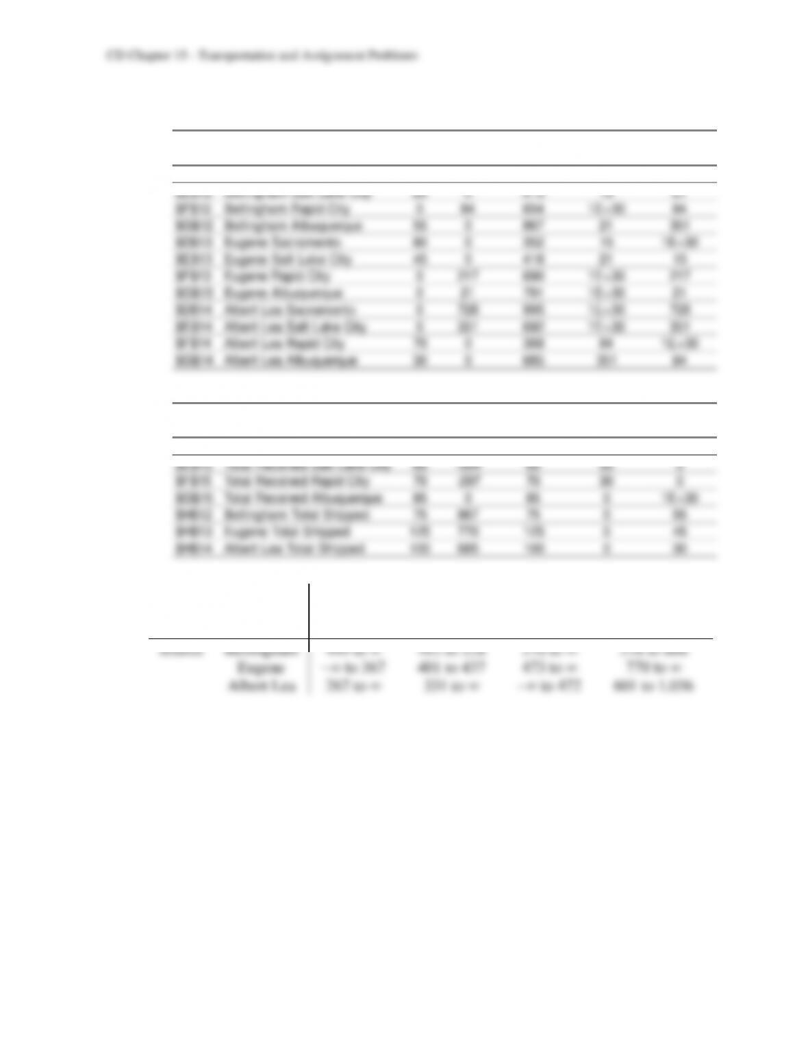
Hauling Cost Site Price
1 2 3 per Ton
Pit North $30 $60 $50 $100
South $60 $30 $40 $120
Unit Cost Site
1 2 3
Pit North $130 $160 $150
South $180 $150 $160
Gravel Hauled Site
1 2 3 Total Supply
Pit North 10 0 8 18 <= 18
South 0 5 2 7 <= 14
Total Received 10 510
= = = Total Cost
Demand 10 510 $3,570
CD15-9
15.9
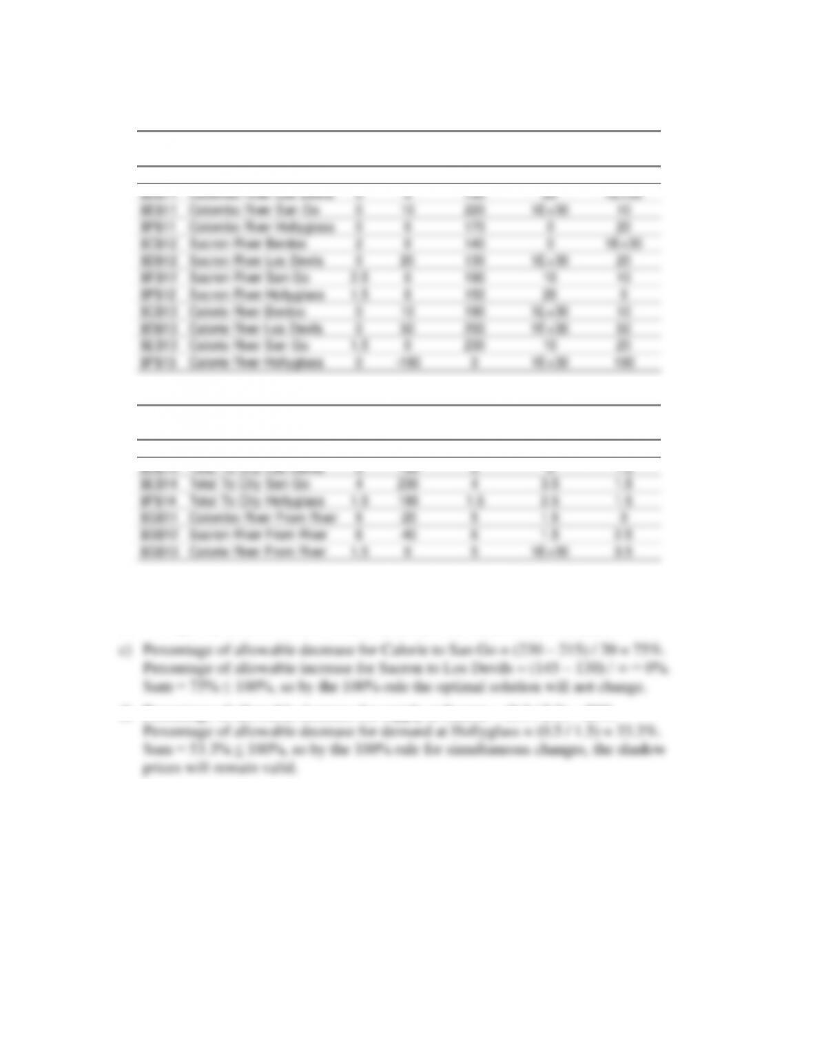
Variable Cells
Final
Reduced
Objective Allowable Allowable
Cell Name Value Cost Coefficient Increase Decrease
$D$12 Bellingham Sacramento 0 15 464 1E+30 15
$E$12 Bellingham Salt Lake City 20 0513 15 21
$F$12 Bellingham Rapid City 0 84 654 1E+30 84
$G$12 Bellingham Albuquerque 55 0867 21 351
$D$13 Eugene Sacramento 80 0352 15 1E+30
$E$13 Eugene Salt Lake City 45 0416 21 15
$F$13 Eugene Rapid City 0 217 690 1E+30 217
$G$13 Eugene Albuquerque 0 21 791 1E+30 21
$D$14 Albert Lea Sacramento 0 728 995 1E+30 728
$E$14 Albert Lea Salt Lake City 0 351 682 1E+30 351
$F$14 Albert Lea Rapid City 70 0388 84 1E+30
$G$14 Albert Lea Albuquerque 30 0685 351 84
Constraints
Final Shadow Constraint Allowable Allowable
Cell Name Value Price R.H. Side Increase Decrease
$D$15 Total Received Sacramento 80 –418 80 45 0
$E$15 Total Received Salt Lake City 65 –354 65 55 0
$F$15 Total Received Rapid City 70 -297 70 30 0
$G$15 Total Received Albuquerque 85 085 0 1E+30
$H$12 Bellingham Total Shipped 75 867 75 055
$H$13 Eugene Total Shipped 125 770 125 045
$H$14 Albert Lea Total Shipped 100 685 100 030
Allowable Range
Destination
Sacramento
Salt Lake City
Rapid City
Albuquerque
Source
Bellingham
449 to ∞
492 to 528
570 to ∞
516 to 888
Eugene
–∞ to 367
401 to 437
473 to ∞
770 to ∞
267 to ∞
601 to 1,036
CD15-10
15.10
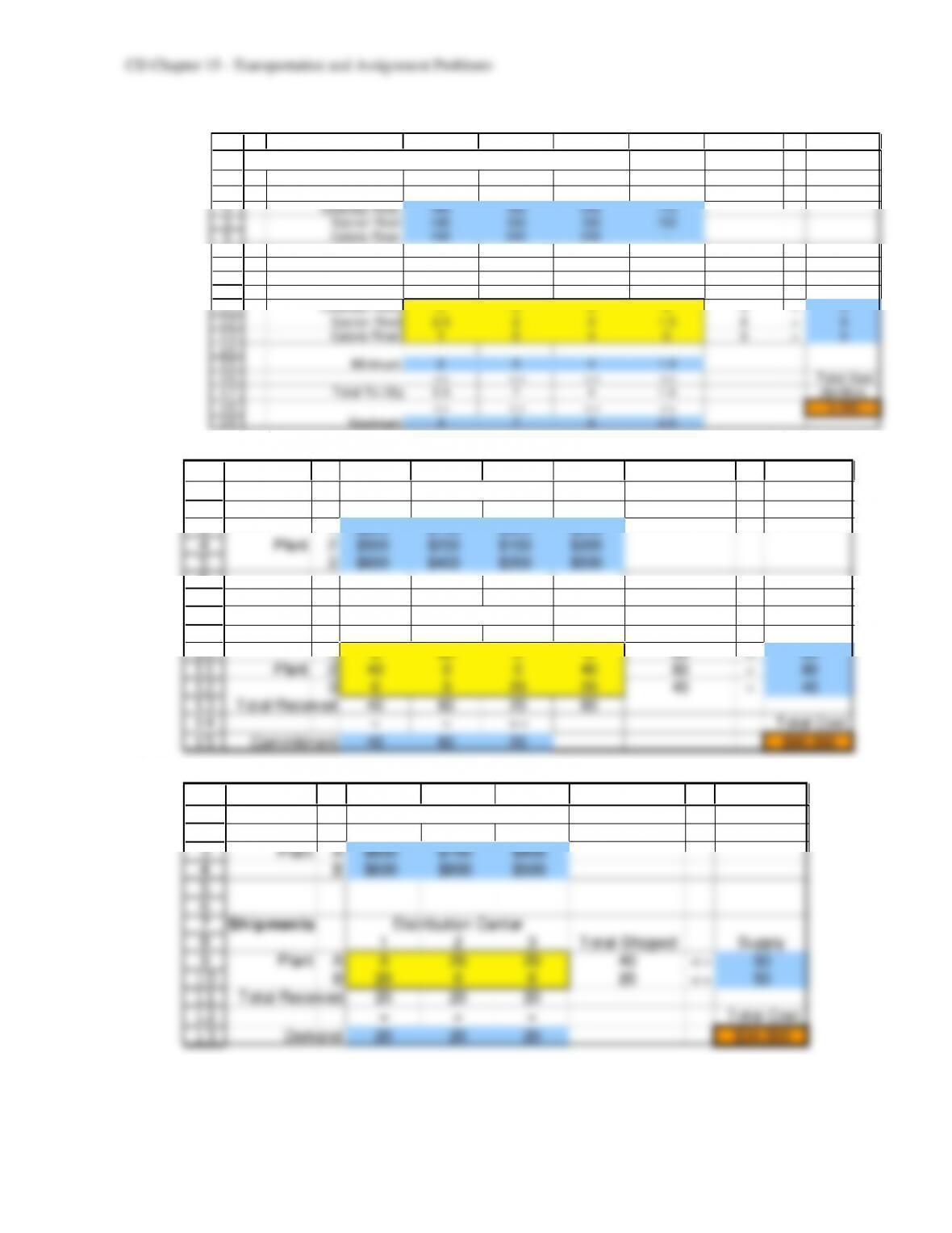
Variable Cells
Final
Reduced
Objective Allowable Allowable
Cell Name Value Cost Coefficient Increase Decrease
$C$11 Colombo River Berdoo 0 0 160 1E+30 0
$D$11 Colombo River Los Devils 5 0 130 20 1E+30
$E$11 Colombo River San Go 0 10 220 1E+30 10
$F$11 Colombo River Hollyglass 0 0 170 020
$C$12 Sacron River Berdoo 2 0 140 0 1E+30
$D$12 Sacron River Los Devils 0 20 130 1E+30 20
$E$12 Sacron River San Go 2.5 0 190 10 10
$F$12 Sacron River Hollyglass 1.5 0 150 20 0
$C$13 Calorie River Berdoo 0 10 190 1E+30 10
$D$13 Calorie River Los Devils 0 50 200 1E+30 50
$E$13 Calorie River San Go 1.5 0 230 10 20
$F$13 Calorie River Hollyglass 0 -190 0 1E+30 190
Constraints
Final Shadow Constraint Allowable Allowable
Cell Name Value Price R.H. Side Increase Decrease
$C$14 Total To City Berdoo 2 180 2 2.5 1.5
$D$14 Total To City Los Devils 5 150 5 0 1.5
$E$14 Total To City San Go 4 230 4 3.5 1.5
$F$14 Total To City Hollyglass 1.5 190 1.5 2.5 1.5
$G$11 Colombo River From River 5 -20 5 1.5 0
$G$12 Sacron River From River 6 –40 6 1.5 2.5
$G$13 Calorie River From River 1.5 0 5 1E+30 3.5
a) The optimal solution would change because the decrease of $30 million is outside the
allowable decrease of $20 million.
b) The optimal solution would remain the same since the allowable increase is ∞.
CD15-11
15.11
1
2
3
4
5
6
7
8
9
10
11
12
13
14
15
16
17
18
19
A B C D E F G H I
Metro W ater District Distribution Problem
Unit Cost ($millions) Berdoo Los Devils San Go Hollyglass
Colombo River 160 130 220 170
Sacron River 140 130 190 150
Calorie River 190 200 230 –
Water Distrib ution Total
(million acre-feet) Berdoo Los Devils San Go Hollyglass From River Available
Colombo River 0 5 0 0 5 = 5
Sacron River 2.5 2 0 1.5 6 = 6
Calorie River 1 0 4 0 5 = 5
Minimum 2 5 4 1.5
<= <= <= <= Total Cost
Total To City 3.5 7 4 1.5 ($million)
<= <= <= <= 2,595
Maximum 4 7 6 3.5
15.12
1
2
3
4
5
6
7
8
9
10
11
12
13
14
15
A B C D E F G H I
Unit Profit
1 2 3 4
1 $800 $700 $500 $200
Plant 2 $500 $200 $100 $300
3 $600 $400 $300 $500
Shipments
1 2 3 4 Total Shipped Supply
1 0 60 0 0 60 =60
Plant 2 40 0 0 40 80 =80
3 0 0 20 20 40 =40
Total Received 40 60 20 60
= = >= Total Cost
Commitment 40 60 20 $90,000
Customer
Customer
15.13
1
2
3
4
5
6
7
8
9
10
11
12
13
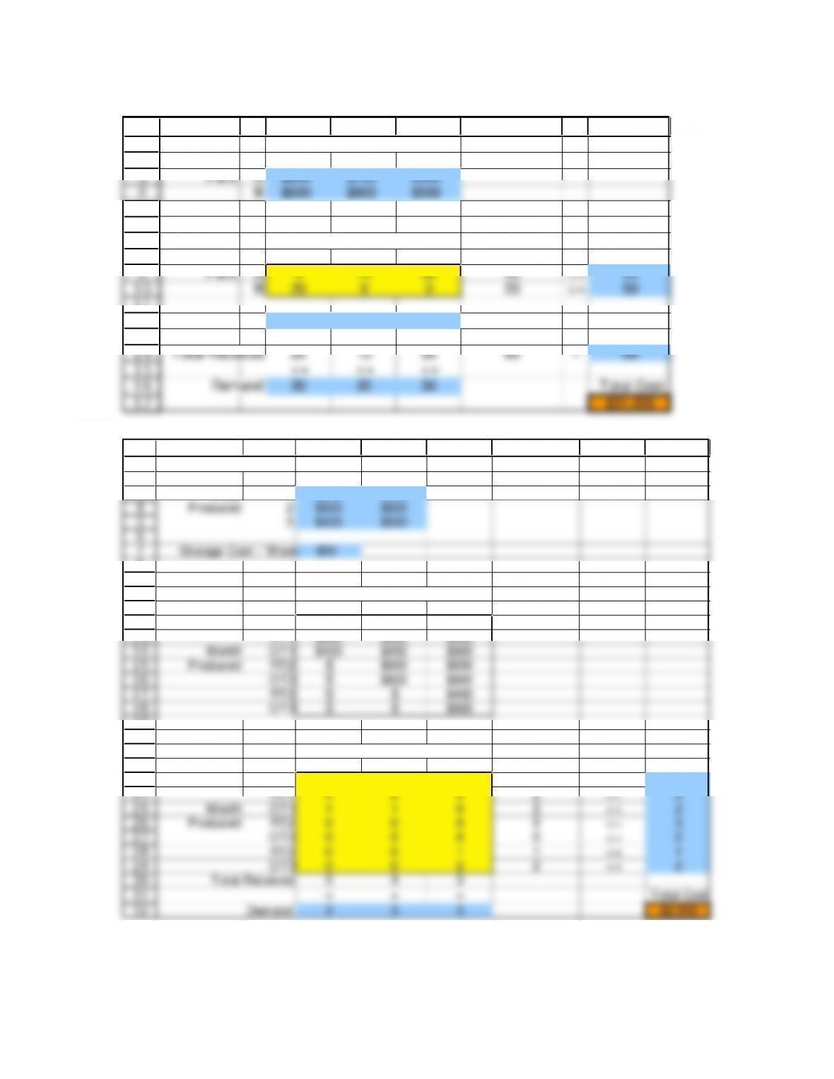
A B C D E F G H
Unit Cost Distribution Center
1 2 3
Plant A $800 $700 $400
B $600 $800 $500
Ship ments Distribution Center
1 2 3 Total Shipped Supply
Plant A 0 20 20 40 <= 50
B20 0 0 20 <= 50
Total Received 20 20 20
= = = Total Cost
Demand 20 20 20 $34,000
CD15-12
15.14
1
2
3
4
5
6
7
8
9
10
11
12
13
14
15
16
17
A B C D E F G H
Unit Cost Distribution Center
1 2 3
Plant A $800 $700 $400
B $600 $800 $500
Shipments Distribution Center
1 2 3 Total Shipped Supply
Plant A 0 10 30 40 <= 50
B20 0 0 20 <= 50
10 10 10
<= <= <= Total
Total Received 20 10 30 60 =60
<= <= <=
Demand 30 30 30 Total Cost
$31,000
15.15
1
2
3
4
5
6
7
8
9
10
11
12
13
14
15
16
17
18
19
20
21
22
23
24
25
26
27
28
29
30
31
32
A B C D E F G H
Production Cost
Regular Overtime
W eek 1 $300 $400
Produced 2 $500 $600
3 $400 $500
Storage Cost / W eek $50
Unit Cost Month Shipped (Product 1)
123
Start $0 $50 $100
RT1 $300 $350 $400
Month OT1 $400 $450 $500
Produced RT2 Š$500 $550
OT2 Š$600 $650
RT3 Š Š $400
OT3 Š Š $500
Shipments W eek Shipped
1 2 3 Total Shipped Capacity
Start 2 0 0 2 = 2
RT1 0 2 0 2 <= 2
Month OT1 1 1 0 2 <= 2
Produced RT2 0 0 0 0 <= 3
OT2 0 0 0 0 <= 2
RT3 0 0 1 1 <= 1
OT3 0 0 2 2 <= 2
Total Received 3 3 3
= = = Total Cost
Demand 3 3 3 $2,950