CD14-1
CD Chapter 14 Solution Concepts for Linear Programming
Review Questions
14.1-1 A corner point is a point that lies at a corner of the feasible region.
14.1-2 The corner point with the best value of the objective function is the optimal solution.
14.1-3 The simplex method has a way of quickly getting to the best corner point and detecting that
this point is optimal, so it stops without needing to evaluate the rest of the corner points.
14.2-1 The best corner point is always an optimal solution.
14.2-2 The big advantage of searching for an optimal solution simply by finding the best corner
point is that it tremendously reduces the number of solutions that need to be considered.
14.2-3 When the simplex method is ready to move from the current corner point to the next one,
the adjacent corner points are candidates to be the next one.
14.3-1 The simplex method focuses solely on solutions that are corner points.
CD14-2
14.3-2 Each iteration of the simplex method consists of a prescribed series of steps for moving
from the current corner point to a new corner point.
14.4-1 No.
14.4-2 The adjacent corner points that are better than the current corner point are candidates to be
the next one.
14.5-1 It is analagous to standing in the middle of a room and looking toward one corner where
two walls and the floor meet.
14.5-2 There are three (at most) adjacent corner points.
14.6-1 The name derives from the fact that the slack variable for a ≤ constraint represents the slack
(gap) between the two sides of the inequality.
14.6-2 A nonnegative slack variable implies that the left-hand side is not larger than the right-hand
side.
CD14-3
14.7-1 (1) Determine the entering basic variable; (2) determine the leaving basic variable;
(3) Solve for the new basic feasible solution
14.7-2 The entering basic variable is the current nonbasic variable that should become a basic
variable for the next basic feasible solution. Among the nonbasic variables with a negative
coefficient in equation 0, choose the one whose coefficient has the largest absolute value to
be the entering basic variable.
14.7-4 The initialization step sets up to start the iterations and finds the initial basic feasible
solution.
14.7-5 Examine the current equation 0. If none of the nonbasic variables have a negative
coefficient, then the current basic feasible solution is optimal.
14.8-1 A problem with several thousand functional constraints and many thousand decision
variables is not considered unusually large for a fast computer.
14.9-1 Narenda Karmarkar.
14.9-2 Today, the more powerful software packages include at least one interior-point algorithm
along with the simplex method.
CD14-4
CD14-5
Problems
14.1
Corner Point (A1, A2)
Profit = $1,000A1 + $2,000A2
(0, 0)
$0
(8, 0)
$8,000
(6, 4)
$14,000
(5, 5)
$15,000
(0, 6.667)
$13,333
14.2
Corner Point (TV, PM)
Cost = TV + 2PM
(0, 9)
$18
(4, 3)
$12
(8, 3)
$14
Optimal Solution: (TV, PM) = (4, 3) and Cost = $12.
14.3 a & d)
1
2
3
4
5
6
7
8
9
10
11
A B C D E F
Activity 1 Activity 2
Unit Profit $30 $20
Used Available
Resource A 1 0 3 <= 5
Resource B 0 1 3 <= 4
Resource C 2 1 9 <= 9
Resource D 3 4 21 <= 21
Activity 1 Activity 2 Total Profit
Number of Units 3 3 $150
Resource Used Per Unit
CD14-6
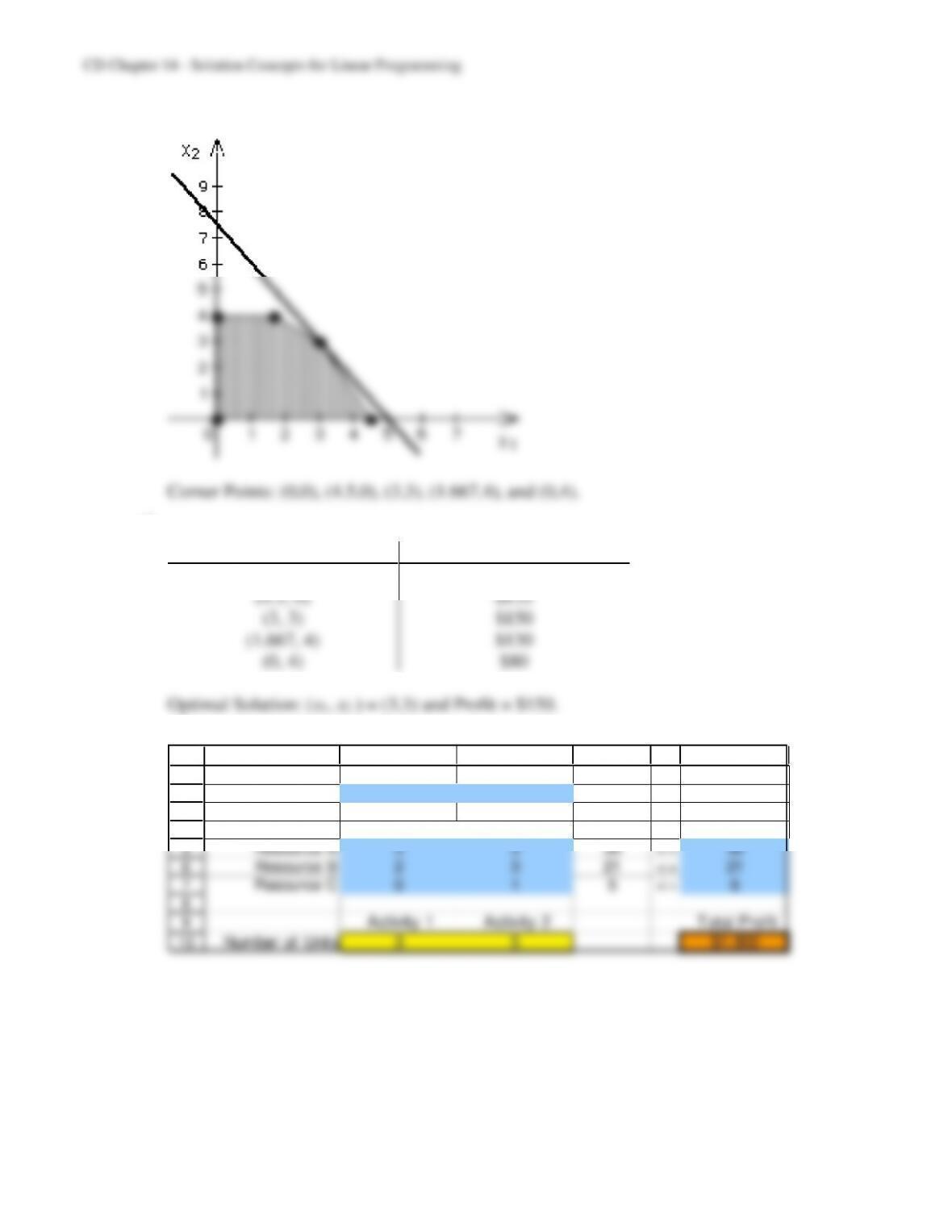
b & e) Optimal Solution: (x1 ,x2 ) = (3, 3) and Profit = $150.
c)
Corner Point (x1, x2)
Profit = $30x1 +$20x2
(0, 0)
$0
(4.5, 0)
$135
(3, 3)
$150
(1.667, 4)
$130
(0, 4)
$80
Optimal Solution: (x1, x2 ) = (3,3) and Profit = $150.
14.4 a & d)
1
2
3
4
5
6
7
8
9
10
A B C D E F
Activity 1 Activity 2
Unit Profit $300 $200
Used Available
Resource A 5 3 30 <= 30
Resource B 2 3 21 <= 21
Resource C 0 1 5 <= 6
Activity 1 Activity 2 Total Profit
Number of Units 3 5 $1,900
Resource Used Per Unit
CD14-7
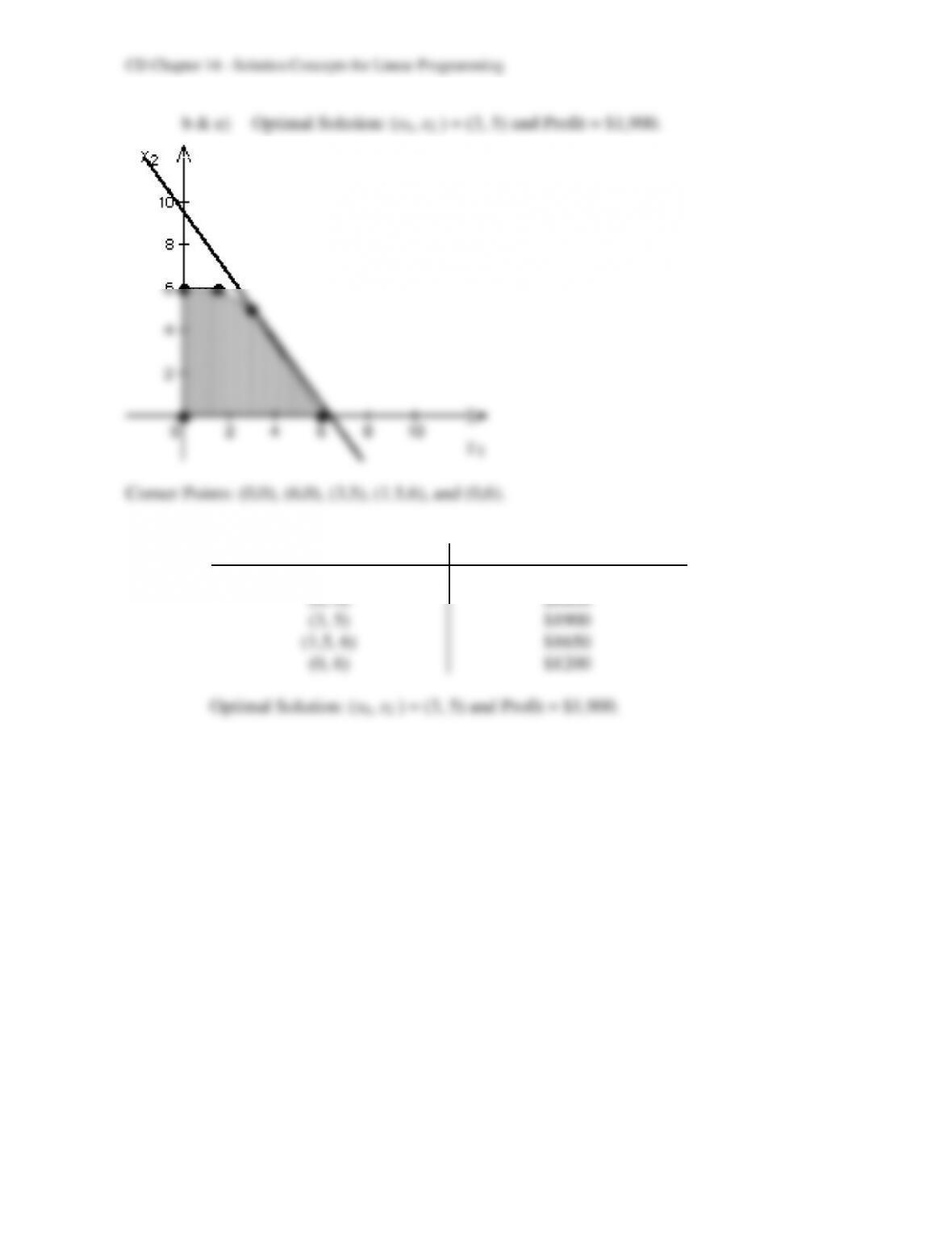
c)
Corner Point (x1, x2)
Profit = $300x1 +$200x2
(0, 0)
$0
(6, 0)
$1800
(3, 5)
$1900
(1.5, 6)
$1650
(0, 6)
$1200
Optimal Solution: (x1, x2 ) = (3, 5) and Profit = $1,900.
CD14-8
CD14-9
CD14-10
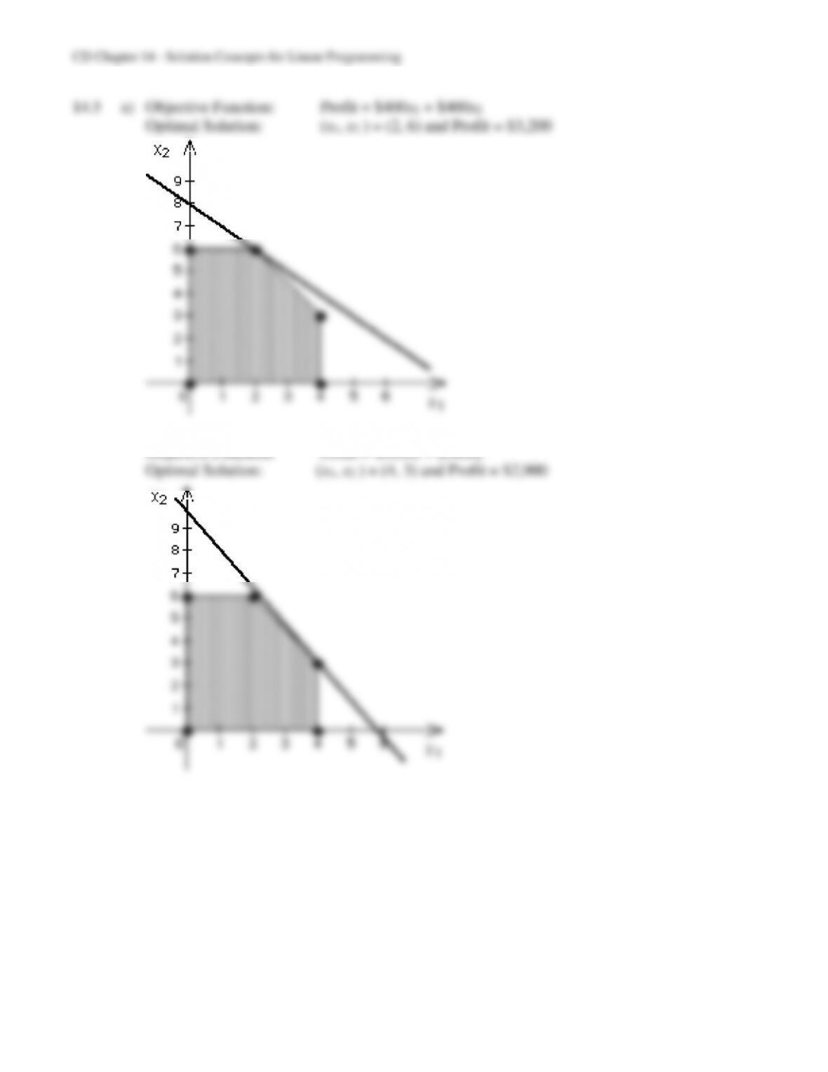
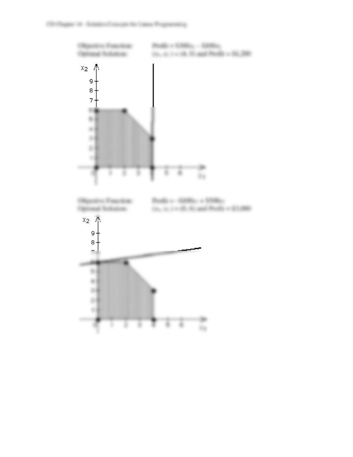
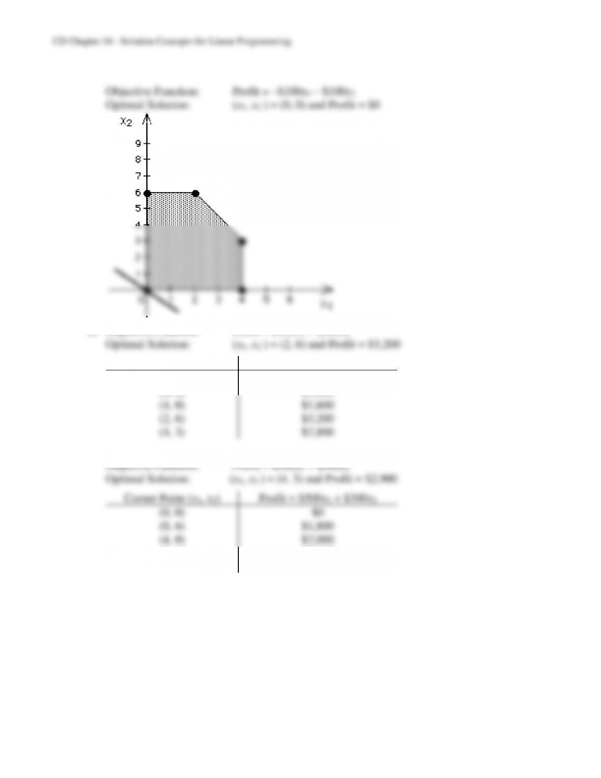
b) Objective Function: Profit = $400x1 + $400x2
Corner Point (x1, x2)
Profit = $400x1 + $400x2
(0, 0)
$0
(0, 6)
$2,400
(4, 0)
$1,600
(2, 6)
$3,200
(4, 3)
$2,800
Corner Point (x1, x2)
Profit = $500x1 + $300x2
(0, 0)
$0
(0, 6)
$1,800
(4, 0)
$2,000
(2, 6)
$2,800
(4, 3)
$2,900
CD14-11
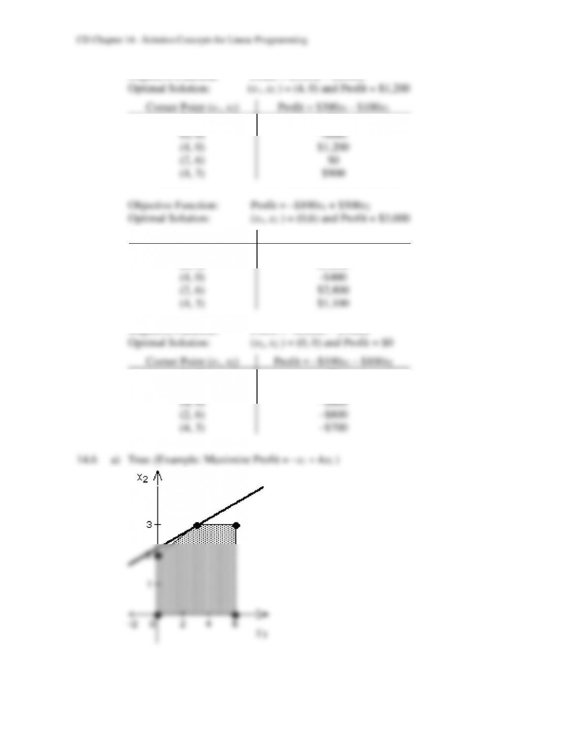
Objective Function: Profit = $300x1 – $100x2
Corner Point (x1, x2)
Profit = $300x1 – $100x2
(0, 0)
$0
(0, 6)
-$600
(4, 0)
$1,200
(2, 6)
$0
(4, 3)
$900
Corner Point (x1, x2)
Profit = -$100x1 + $500x2
(0, 0)
$0
(0, 6)
$3,000
(4, 0)
-$400
(2, 6)
$2,800
(4, 3)
$1,100
Objective Function: Profit = –$100x1 – $100x2
Corner Point (x1, x2)
Profit = –$100x1 – $100x2
(0, 0)
$0
(0, 6)
–$600
(4, 0)
–$400
(2, 6)
–$800
(4, 3)
–$700
CD14-12
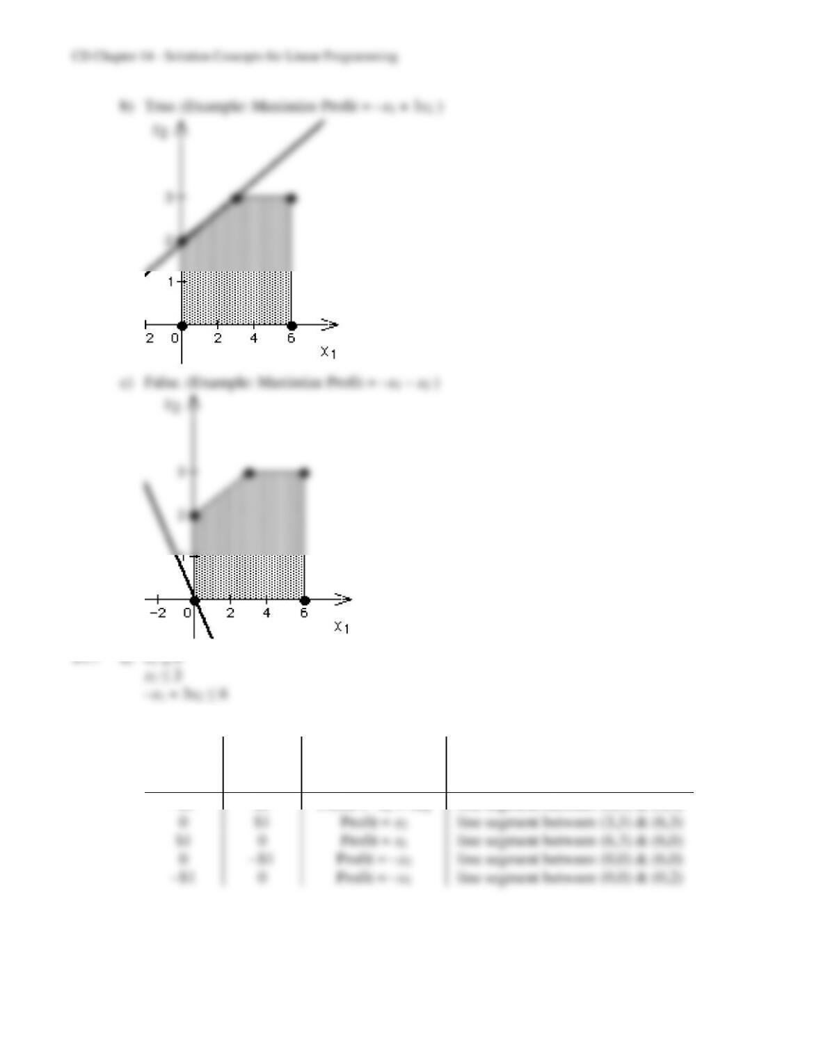
b)
Unit
Profit
Product 1
Unit
Profit
Product 2
Objective Function
Multiple Optimal Solutions
–$1
$3
Profit = –x1 + 3x2
line segment between (0,2) & (3,3)
0
$1
Profit = x2
line segment between (3,3) & (6,3)
$1
0
Profit = x1
line segment between (6,3) & (6,0)
0
–$1
Profit = –x2
line segment between (0,0) & (6,0)
–$1
0
Profit = –x1
line segment between (0,0) & (0,2)
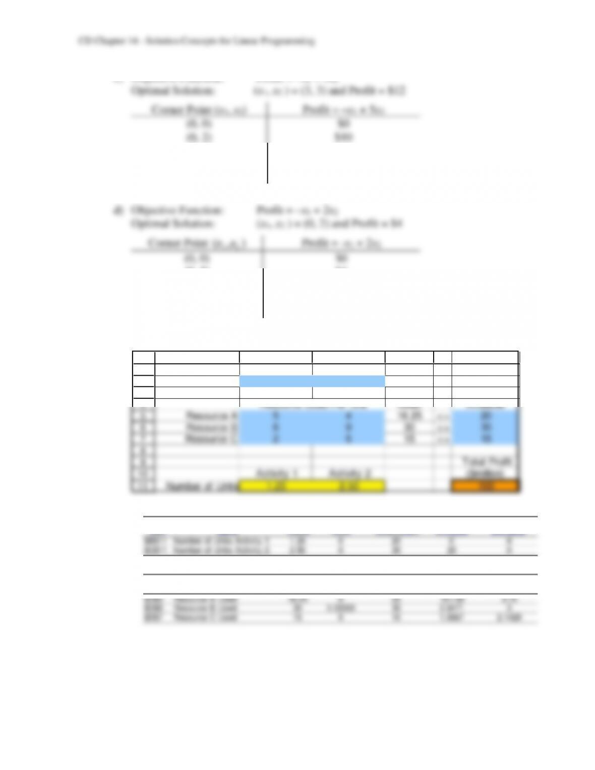
c) Objective Function: Profit = –x1 + 5x2
CD14-14
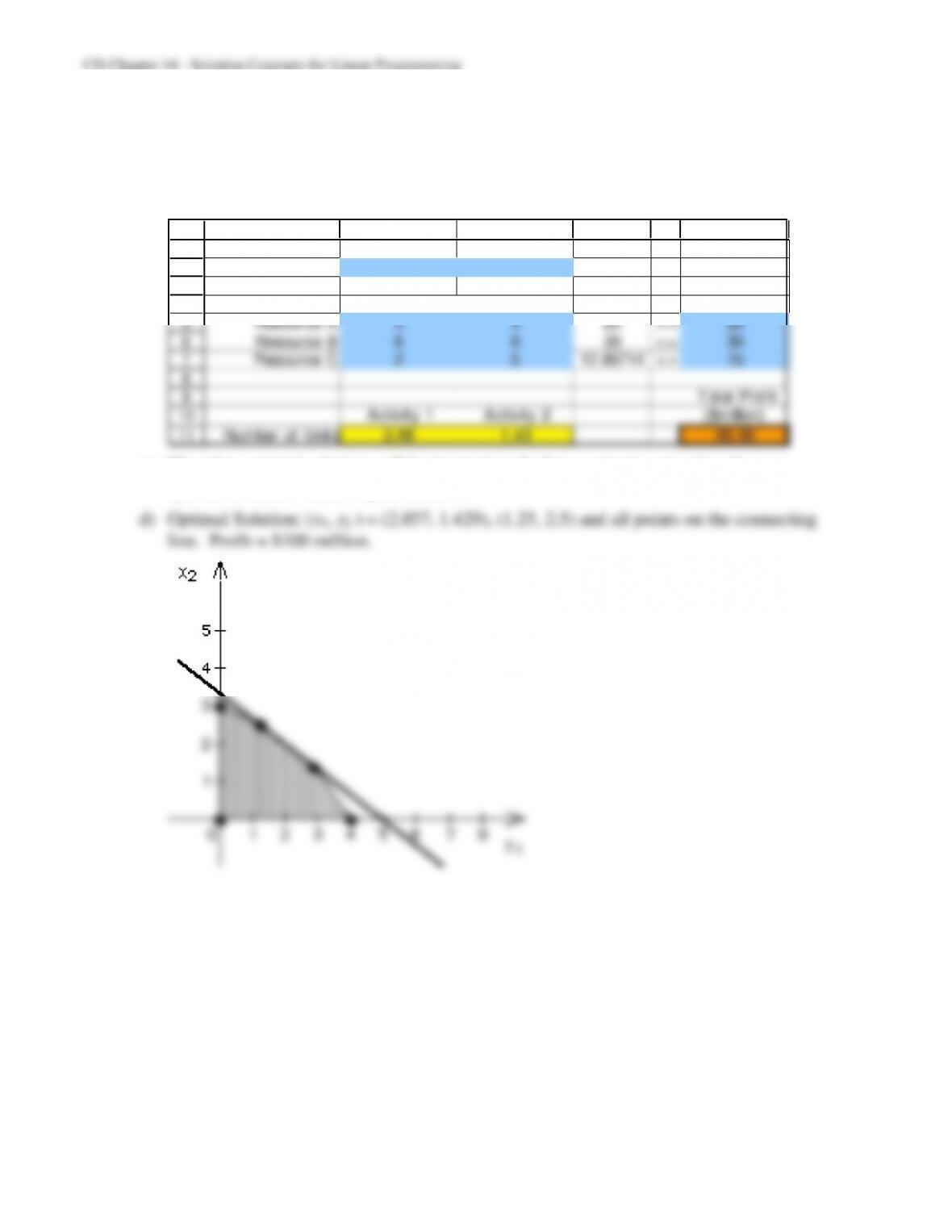
b) The sensitivity report indicates that the problem has other optimal solutions because the
allowable increase of Activity 1 and the allowable decrease of Activity 2 are 0. An
alternative optimal solution is shown below (obtained by adjusting the unit profit for
Activity 2 to 29.99).
1
2
3
4
5
6
7
8
9
10
11
A B C D E F
Activity 1 Activity 2
Unit Profit 20 29.99 ($million)
Used Available
Resource A 5 4 20 <= 20
Resource B 6 9 30 <= 30
Resource C 2 5 12.85714 <= 15
Total Profit
Activity 1 Activity 2 ($million)
Number of Units 2.86 1.43 99.99
Resource Used Per Unit
c) The other optimal solutions will be located on the line segment connecting the two
optimal solutions found in parts a and b.
CD14-15
14.9 a)
1
2
3
4
5
6
7
8
9
10
A B C D E F
Activity 1 Activity 2
Unit Profit $500 $300
Used Available
Resource A 15 5 300 <= 300
Resource B 10 6 240 <= 240
Resource C 8 12 300 <= 450
Activity 1 Activity 2 Total Profit
Number of Units 15 15 $12,000
Resource Used Per Unit
Adjustable Cells
Final Reduced Objective Allowable Allo w able
Cell Name Value Cost Coefficient Increase Decrease
$B$10 Number of Units Activity 1 15.00 0.00 500 400 0
$C$10 Number of Units Activity 2 15.00 0.00 300 0 133.3333
Constraints
Final Shadow Constraint Allo w able Allo w able
Cell Name Value Price R.H. Side Increase Decrease
$D$5 Resource A Used 300 0 300 60 83.3333
$D$6 Resource B Used 240 50 240 42.8571 40
$D$7 Resource C Used 300 0 450 1E+ 30 150
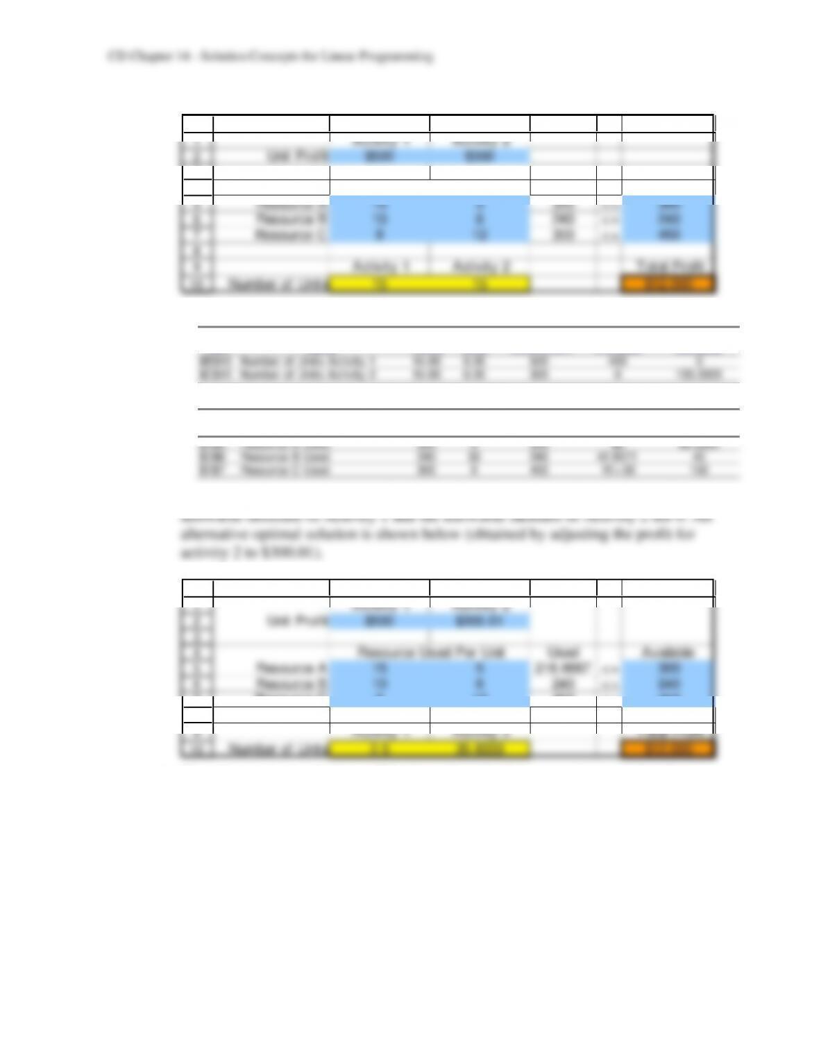
b) The sensitivity report indicates that the problem has other optimal solutions because the
1
2
3
4
5
6
7
8
9
10
A B C D E F
Activity 1 Activity 2
Unit Profit $500 $300.01
Used Available
Resource A 15 5 216.6667 <= 300
Resource B 10 6 240 <= 240
Resource C 8 12 450 <= 450
Activity 1 Activity 2 Total Profit
Number of Units 2.5 35.8333 $12,000
Resource Used Per Unit
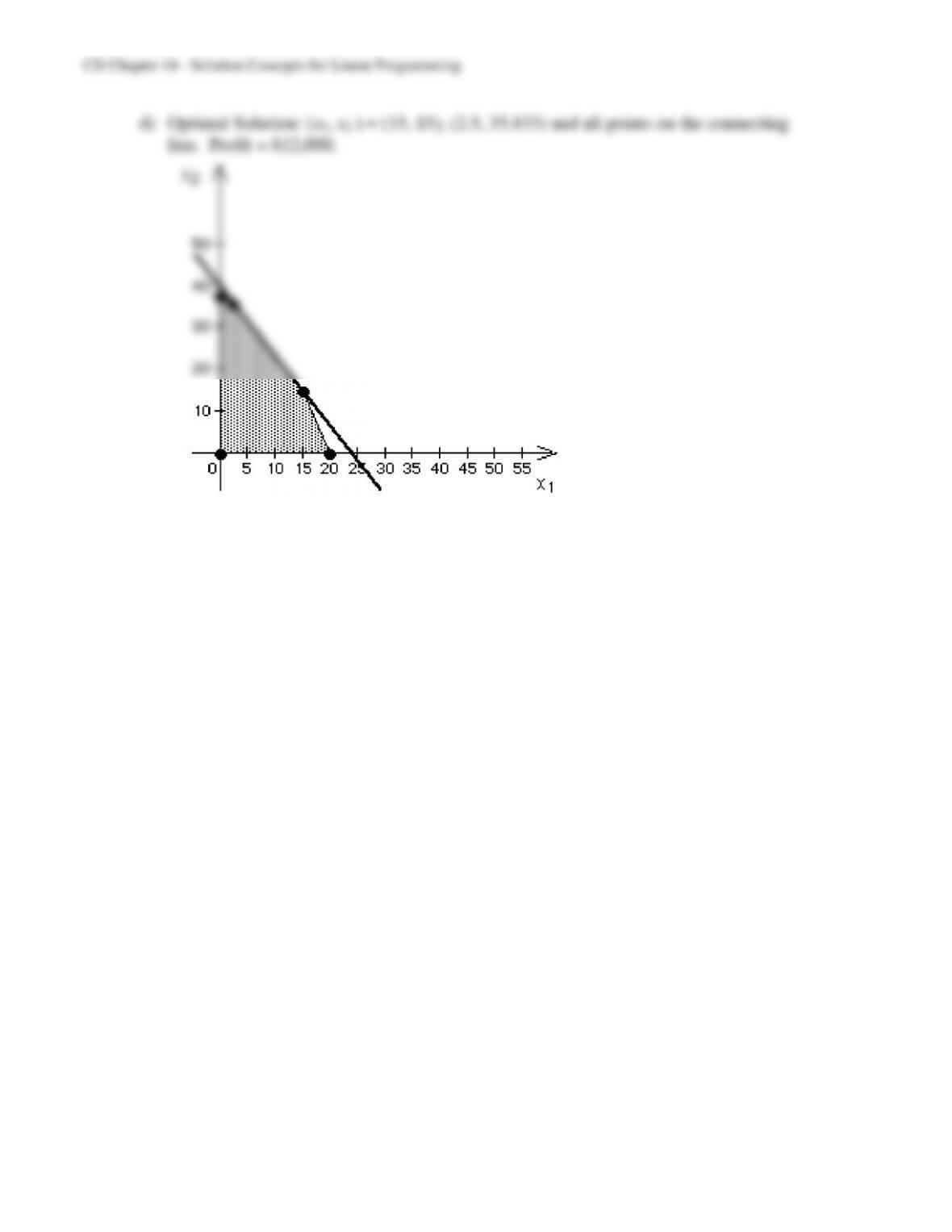
c) The other optimal solutions will be located on the line segment connecting the two
optimal solutions found in parts a) and b).
CD14-16
CD14-17
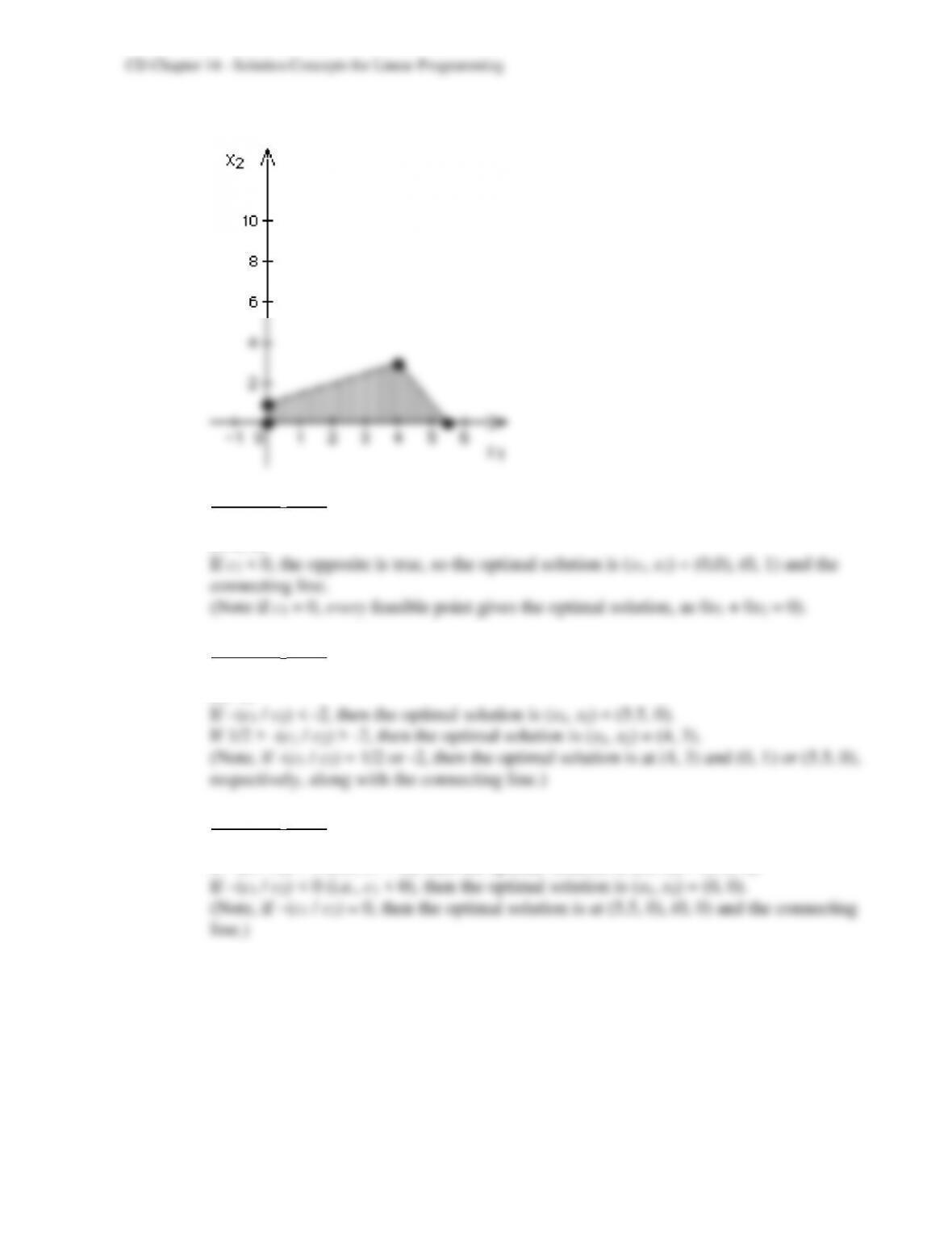
14.10 Feasible Region:
Case 1 (c2 = 0):
If c1 > 0, the objective increases as x1 increases, so the optimal solution is (x1, x2) =
(5.5, 0).
Case 2 (c2 > 0): (slope of objective function line is –(c1 / c2))
If –(c1 / c2) > 1/2 (or equivalently, c1/c2 < –1/2), then the optimal solution is (x1, x2) =
(0, 1).
Case 3 (c2 < 0): (slope of objective function line is still -(c1 / c2), but the objective
function value increases as the line is shifted down)
If –(c1 / c2) > 0 (i.e., c1 > 0), then the optimal solution is (x1, x2) = (5.5, 0).
CD14-18
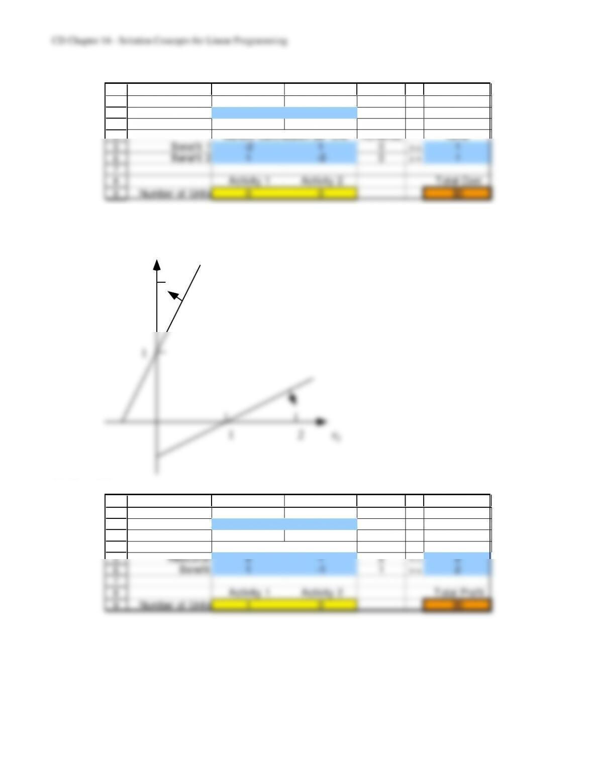
14.11 a & b)
1
2
3
4
5
6
7
8
9
A B C D E F
Activity 1 Activity 2
Unit Cost $5,000 $7,000 Minimum
Benefit Acceptable
Achieved Level
Benefit 1 -2 1 0 >= 1
Benefit 2 1 -2 0>= 1
Activity 1 Activity 2 Total Cost
Number of Units 0 0 $0
Benefit Contribution per Unit
Solver could not find a feasible solution.
c)
1 2
1
2
x1
x2
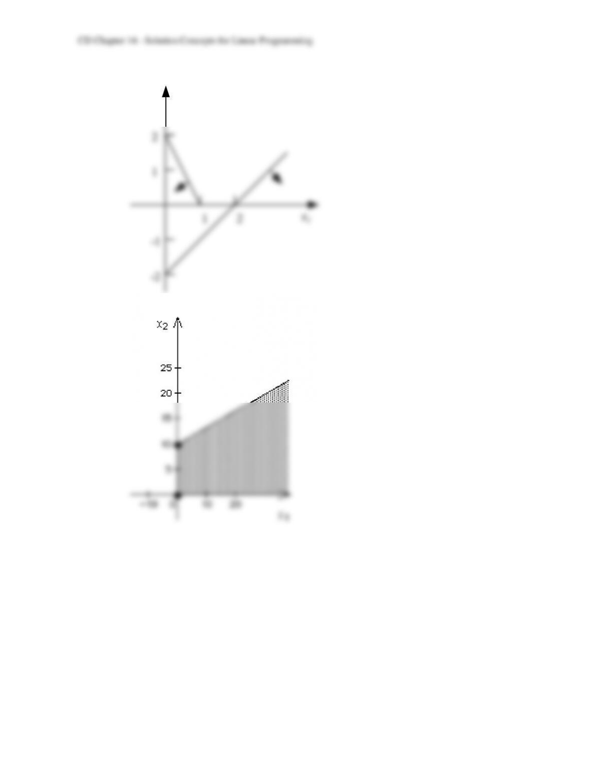
14.12 a & b)
1
2
3
4
5
6
7
8
9
A B C D E F
Activity 1 Activity 2
Unit Profit 90 70
Available/
Level Minimum
Resource 2 1 2 <= 2
Benefit 1 -1 1>= 2
Activity 1 Activity 2 Total Profit
Number of Units 1 0 90
Benefit Contribution per Unit
Solver could not find a feasible solution.
CD14-19
c)
1 2
2
-2
x1
x2
-1
1
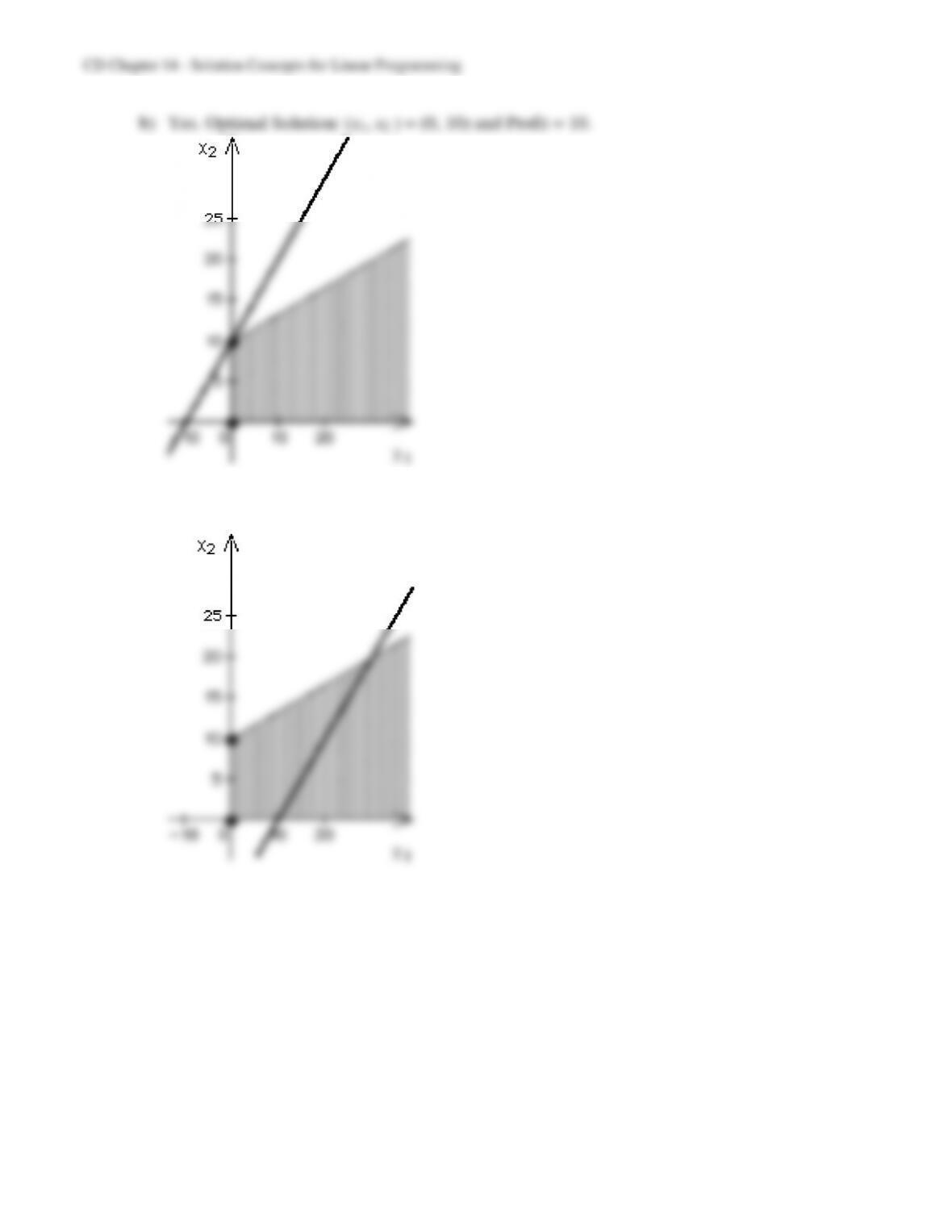
14.13 a)
CD14-20
c) No. The objective function value is maximized by sliding the objective function line to
the right. This can be done forever, so there is no optimal solution.
d) No, solutions exist that will make the profit arbitrarily large. This usually occurs when
a constraint is left out of the model.