13–38
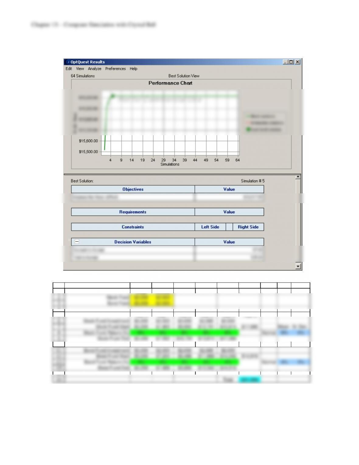
c) They should accept approximately 67 discount reservations and up to approximately
125 total in order to maximize mean profit, as found by OptQuest.
13.23
1
2
3
4
5
6
7
8
9
10
11
12
13
14
15
16
A B C D E F G H I J
Initial Annual
Stock Fund $3,000 $2,000
Bond Fund $3,000 $2,000
Year 0 Year 1 Year 2 Year 3 Year 4 Year 5
Stock Fund Investment $5,000 $2,000 $2,000 $2,000 $2,000
Stock Fund Start $5,000 $7,400 $9,992 $12,791 $15,815 $17,080 Mean St. Dev.
Stock Fund Return (%) 8% 8% 8% 8% 8% Normal 8% 6%
Stock Fund End $5,400 $7,992 $10,791 $13,815 $17,080
Bond Fund Investment $5,000 $2,000 $2,000 $2,000 $2,000
Bond Fund Start $5,000 $7,200 $9,488 $11,868 $14,342 $14,916
Bond Fund Return (%) 4% 4% 4% 4% 4% Normal 4% 3%
Bond Fund End $5,200 $7,488 $9,868 $12,342 $14,916
13–39
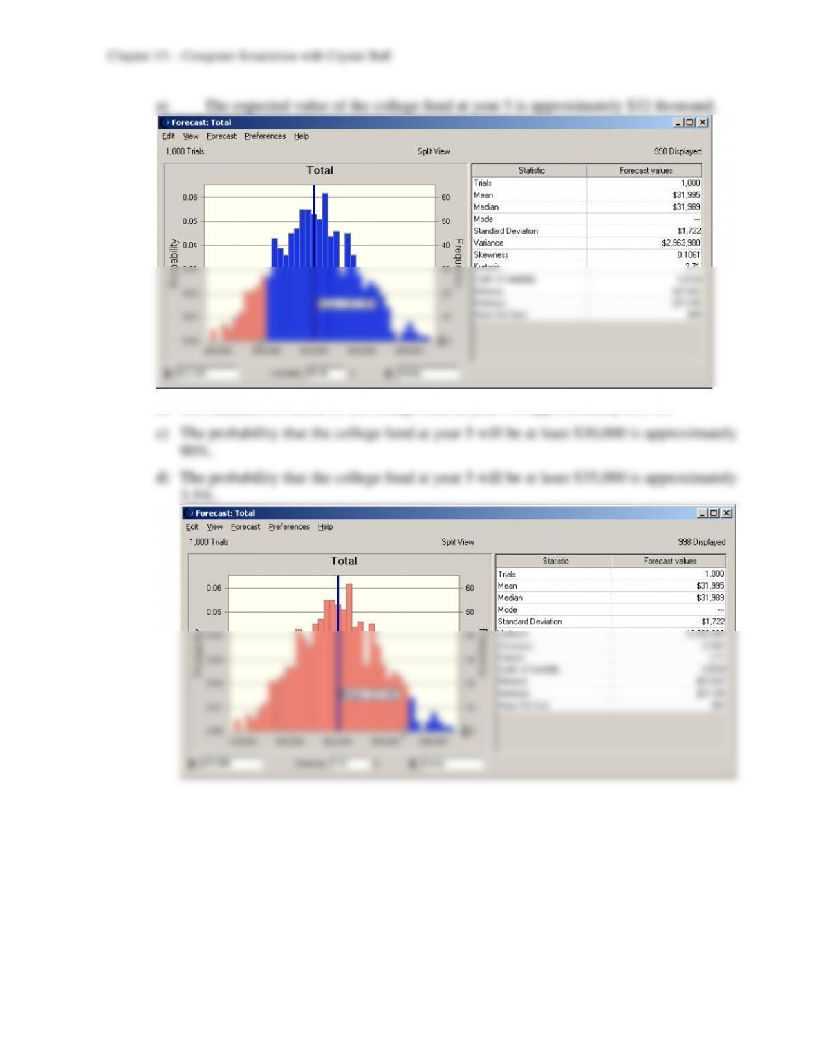
b) The standard deviation of the college fund at year 5 is approximately $1,700.
13–40
Cases
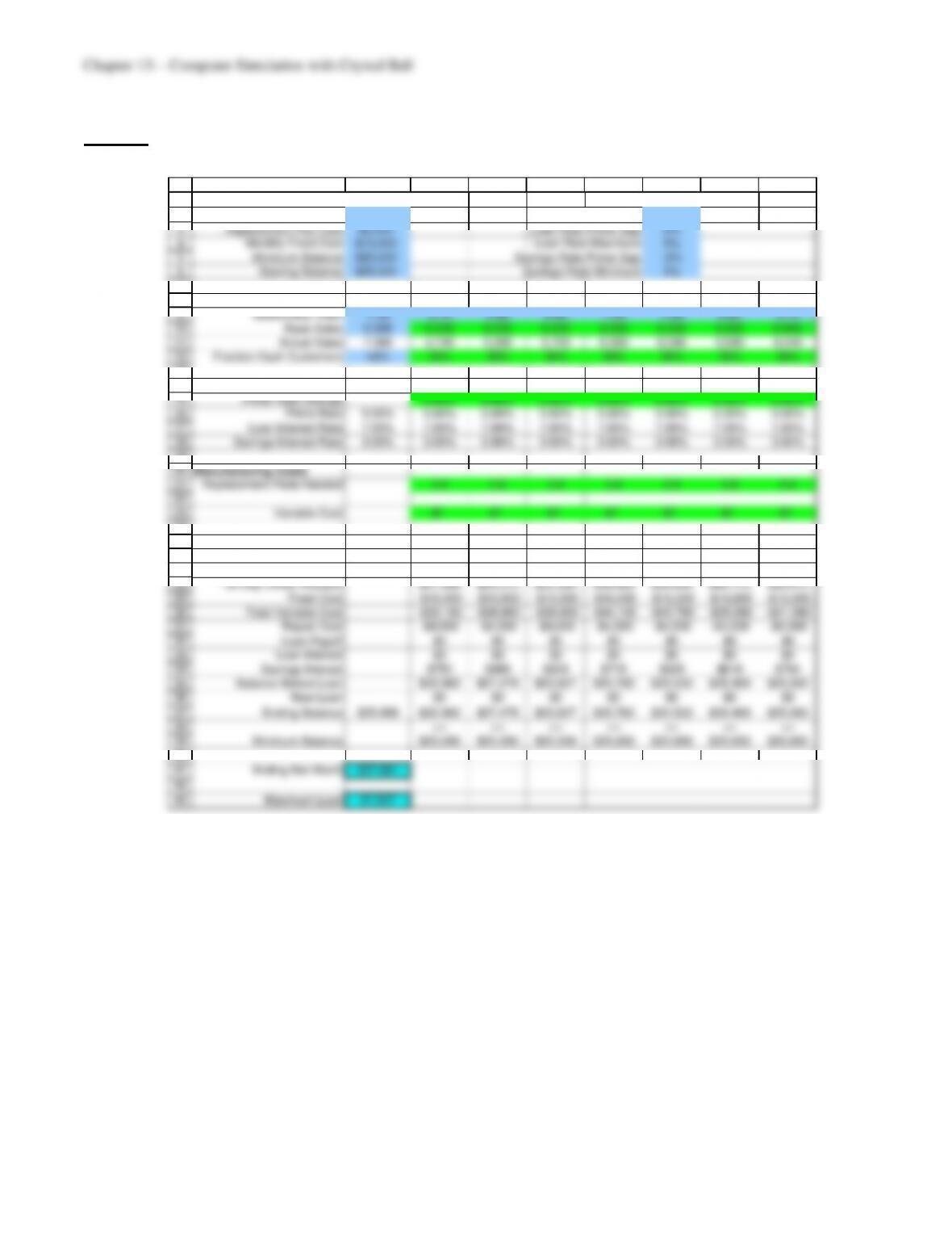
13.1 a) The spreadsheet model is spread over the next several pages:
1
2
3
4
5
6
7
8
9
10
11
12
13
14
15
16
17
18
19
20
21
22
23
24
25
26
27
28
29
30
31
32
36
37
38
40
41
42
43
A B C D E F G H I
Cost & Revenue Data Interest Rate Data
Selling Price $10 Initial Prime Rate 5%
Replacement Part Cost $5,000 Loan Rate Prime Gap 2%
Monthly Fixed Cost $15,000 Loan Rate Maximum 9%
Minimum Balance $20,000 Savings Rate Prime Gap -2%
Starting Balance $25,000 Savings Rate Minimum 2%
Sales Dec Jan Feb Mar Apr May June July
Seasonality Index 1.18 0.79 0.88 0.95 1.05 1.09 0.84 0.74
Base Sales 6,000 6,000 6,000 6,000 6,000 6,000 6,000 6,000
Actual Sales 7,080 4,740 5,280 5,700 6,300 6,540 5,040 4,440
Fraction Cash Customers 42% 39% 39% 39% 39% 39% 39% 39%
Interest Rates
Prime Rate Change 0.00% 0.00% 0.00% 0.00% 0.00% 0.00% 0.00%
Prime Rate 5.00% 5.00% 5.00% 5.00% 5.00% 5.00% 5.00% 5.00%
Loan Interest Rate 7.00% 7.00% 7.00% 7.00% 7.00% 7.00% 7.00% 7.00%
Savings Interest Rate 3.00% 3.00% 3.00% 3.00% 3.00% 3.00% 3.00% 3.00%
Manufacturing Costs
Replacement Parts Needed 0.8 0.8 0.8 0.8 0.8 0.8 0.8
Variable Cost $7 $7 $7 $7 $7 $7 $7
Cash Flows
Beginning Balance $25,000 $32,962 $27,479 $23,827 $20,762 $20,533 $26,469
Cash Receipts $18,328 $20,416 $22,040 $24,360 $25,288 $19,488 $17,168
30-Day Credit Receipts $41,064 $29,072 $32,384 $34,960 $38,640 $40,112 $30,912
Fixed Cost -$15,000 -$15,000 -$15,000 -$15,000 -$15,000 -$15,000 -$15,000
Total Variable Cost -$33,180 -$36,960 -$39,900 -$44,100 -$45,780 -$35,280 -$31,080
Repair Cost -$4,000 -$4,000 -$4,000 -$4,000 -$4,000 -$4,000 -$4,000
Loan Payoff $0 $0 $0 $0 $0 $0 $0
Ending Balance $25,000 $32,962 $27,479 $23,827 $20,762 $20,533 $26,469 $25,263
>= >= >= >= >= >= >=
Maximum Loan $7,507
13–41
1
2
3
4
5
6
7
8
9
10
11
12
13
14
15
16
17
18
19
20
21
22
23
24
25
26
27
28
29
30
31
32
33
34
35
36
37
38
39
40
41
42
43
A B C
Cost & Revenue Data
Selling Price 10
Replacement Part Cost 5000
Monthly Fixed Cost 15000
Minimum Balance 20000
Starting Balance 25000
Sales Dec Jan
Seasonality Index 1.18 0.79
Base Sales 6000 6000
Actual Sales =SeasonalityIndex*BaseSales =SeasonalityIndex*BaseSales
Fraction Cash Customers 0.42 0.386666666666667
Interest Rates
Prime Rate Change 1.6784487245436E-19
Prime Rate =InitialPrimeRate =B16+PrimeRateChange
Loan Interest Rate =MIN(PrimeRate+LoanRateGap,LoanRateMax) =MIN(PrimeRate+LoanRateGap,LoanRateMax)
Savings Interest Rate =MAX(PrimeRate+SavingsRateGap,SavingsRateMin) =MAX(PrimeRate+SavingsRateGap,SavingsRateMin)
Manufacturing Costs
Replacement Parts Needed 0.8
Variable Cost 7
Cash Flows
Beginning Balance =B37
Cash Receipts =ActualSales*FractionCashCustomers*SellingPrice
30-Day Credit Receipts =B11*(1-B12)*SellingPrice
Fixed Cost =-MonthlyFixedCost
Total Variable Cost =-VariableCost*ActualSales
Repair Cost =-ReplacementPartsNeeded*ReplacementPartCost
Loan Payoff =-B36
Loan Interest =-B36*B17
Savings Interest =B37*B18
Balance Before Loan =SUM(C26:C34)
New Loan =IF(BalanceBeforeLoan<=MinimumBalance,MinimumBalance-BalanceBeforeLoan,0)
Ending Balance =StartingBalance =BalanceBeforeLoan+NewLoan
>=
Minimum Balance =MinimumBalance
Ending Net Worth =O35
Maximum Loan =MAX(NewLoan)
13–42
41
42
43
1
2
3
4
5
6
7
8
9
10
11
12
13
14
15
16
17
18
19
20
21
22
23
24
25
26
27
28
29
30
31
32
33
34
35
36
37
38
39
40
A J K L M N O P Q R
Selling Price
Replacement Part Cost
Monthly Fixed Cost
Minimum Balance
Starting Balance
Sales August Sept October November December January
Seasonality Index 0.98 1.06 1.1 1.16 1.18
Base Sales 6,000 6,000 6,000 6,000 6,000 Normal prev mo. 500
Actual Sales 5,880 6,360 6,600 6,960 7,080
Fraction Cash Customers 39% 39% 39% 39% 39% Triangular 28% 40% 48%
Interest Rates
Prime Rate Change 0.00% 0.00% 0.00% 0.00% 0.00% Custom -0.50% 0.05
Prime Rate 5.00% 5.00% 5.00% 5.00% 5.00% -0.25% 0.1
Loan Interest Rate 7.00% 7.00% 7.00% 7.00% 7.00% 0% 0.7
Savings Interest Rate 3.00% 3.00% 3.00% 3.00% 3.00% 0.25% 0.1
0.50% 0.05
Manufacturing Costs
Replacement Parts Needed 0.8 0.8 0.8 0.8 0.8 Binomial 10% 8
Variable Cost $7 $7 $7 $7 $7 Uniform $6 $8
Cash Flows
Beginning Balance $25,263 $20,000 $20,000 $20,000 $20,000 $20,000
Cash Receipts $22,736 $24,592 $25,520 $26,912 $27,376
30-Day Credit Receipts $27,232 $36,064 $39,008 $40,480 $42,688 $43,424
Fixed Cost -$15,000 -$15,000 -$15,000 -$15,000 -$15,000
Total Variable Cost -$41,160 -$44,520 -$46,200 -$48,720 -$49,560
Repair Cost -$4,000 -$4,000 -$4,000 -$4,000 -$4,000
Loan Payoff $0 -$4,171 -$6,727 -$7,270 -$7,507 -$5,928
Loan Interest $0 -$292 -$471 -$509 -$525 -$415
Savings Interest $758 $600 $600 $600 $600 $600
Balance Before Loan $15,829 $13,273 $12,730 $12,493 $14,072 $57,681
New Loan $4,171 $6,727 $7,270 $7,507 $5,928
Ending Balance $20,000 $20,000 $20,000 $20,000 $20,000
>= >= >= >= >=
Minimum Balance $20,000 $20,000 $20,000 $20,000 $20,000
1
2
3
4
5
6
7
8
9
10
11
12
13
14
15
16
17
18
19
20
21
22
23
24
25
26
27
28
29
30
31
32
33
34
35
36
37
38
39
40
41
42
43
A N O
Selling Price
Replacement Part Cost
Monthly Fixed Cost
Minimum Balance
Starting Balance
Sales December January
Seasonality Index 1.18
Base Sales 6000 Normal
Actual Sales =SeasonalityIndex*BaseSales
Fraction Cash Customers 0.386666666666667 Triangular
Interest Rates
Prime Rate Change 1.6784487245436E-19 Custom
Prime Rate =M16+PrimeRateChange
Loan Interest Rate =MIN(PrimeRate+LoanRateGap,LoanRateMax)
Savings Interest Rate =MAX(PrimeRate+SavingsRateGap,SavingsRateMin)
Manufacturing Costs
Replacement Parts Needed 0.8 Binomial
Variable Cost 7 Uniform
Cash Flows
Beginning Balance =M37 =N37
Cash Receipts =ActualSales*FractionCashCustomers*SellingPrice
30-Day Credit Receipts =M11*(1-M12)*SellingPrice =N11*(1-N12)*SellingPrice
Fixed Cost =-MonthlyFixedCost
Total Variable Cost =-VariableCost*ActualSales
Repair Cost =-ReplacementPartsNeeded*ReplacementPartCost
Loan Payoff =-M36 =-N36
Loan Interest =-M36*M17 =-N36*N17
Savings Interest =M37*M18 =N37*N18
Balance Before Loan =SUM(N26:N34) =SUM(O26:O34)
New Loan =IF(BalanceBeforeLoan<=MinimumBalance,MinimumBalance-BalanceBeforeLoan,0)
Ending Balance =BalanceBeforeLoan+NewLoan
>=
Minimum Balance =MinimumBalance
Ending Net Worth
Maximum Loan
13–44
The range names are as follows:
Range Name Cells
ActualSales B11:N11
BalanceBeforeLoan C35:N35
BaseSales B10:N10
BeginningBalance C26:N26
CashReceipts C27:N27
CreditReceipts C28:N28
EndingBalance C37:N37
EndingNetW orth B41
FixedCost C29:N29
FractionCashCustomers B12:N12
InitialPrimeRate G2
LoanInterest C33:N33
LoanPayoff C32:N32
LoanRate B17:N17
LoanRateGap G3
LoanRateMax G4
MaximumLoan B43
MinimumBalance B5
MonthlyFixedCost B4
NewLoan C36:N36
13–45
c) The maximum short-term loan is forecasted in cell B43. The cumulative chart and
percentile chart follow. These charts indicate that the maximum short-term loan
13–46
13.2 a) Before we begin the formal problem, we must first calculate the mean
and standard
deviation
of the normally distributed random variable N. We are told that the annual
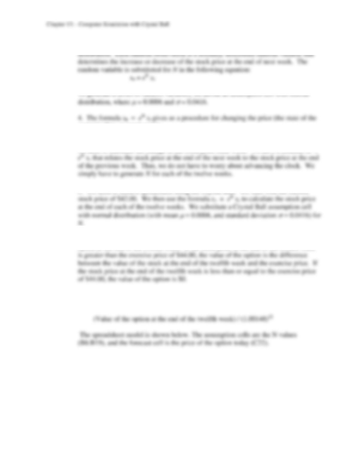
We first convert the annual interest rate r = 8% to a weekly interest rate w with the
following formula:
We next convert the annual volatility Va = 0.30 to a weekly volatility Vw with the
following formula:
Once we have the weekly interest rate and volatility, we can calculate
and
.
1. One component appears in this system: the stock price. The stock price in the
previous week is used to calculate the stock price in the next week. The relationship
13–47
3. This simulation requires generating a series of random observations from the normal
system) when an event occurs.
5. In this simulation, the time periods are fixed. We have a twelve-week period, and
we need to calculate the change in the stock price each week. We have a formula sn =
6. We need to build a spreadsheet using the Crystal Ball. We start with the current
We then use the stock price at the end of the twelfth week to calculate the value of the
option at the end of the twelfth week. If the stock price at the end of the twelfth week
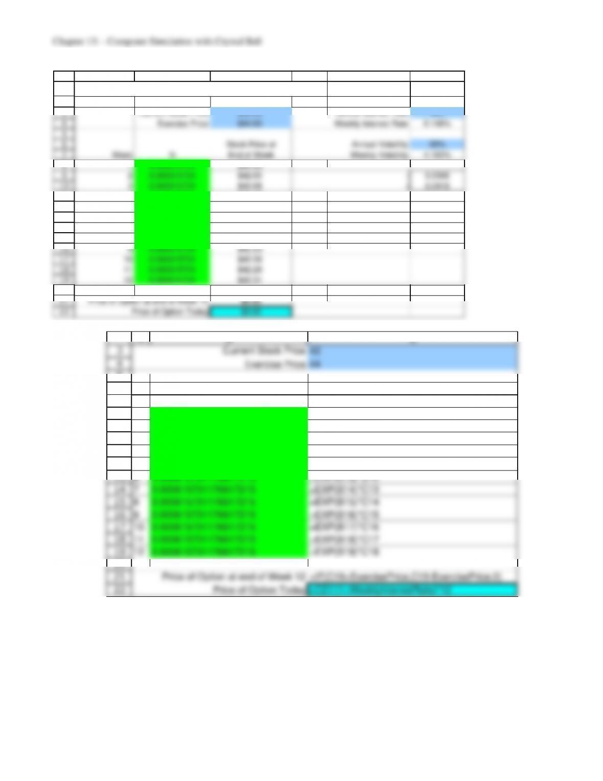
Finally, we need to discount the value of the option at the end of the twelfth week to the
value of the option in today’s dollars using the following formula:
22
1
2
3
4
5
6
7
8
9
10
11
12
13
14
15
16
17
18
19
20
21
22
A B C D E F
Simulation Model to Estimate Option Value
Current Stock Price $42.00 Annual Interest Rate 8%
Exercise Price $44.00 Weekly Interest Rate 0.148%
Stock Price at Annual Volatility 30%
Week N End of Week Weekly Volatility 4.160%
1 0.000615731 $42.03
2 0.000615731 $42.05
m = 0.0006
3 0.000615731 $42.08
s = 0.0416
4 0.000615731 $42.10
5 0.000615731 $42.13
6 0.000615731 $42.16
7 0.000615731 $42.18
8 0.000615731 $42.21
9 0.000615731 $42.23
10 0.000615731 $42.26
11 0.000615731 $42.29
12 0.000615731 $42.31
Price of Option at end of Week 12 $0.00
Price of Option Today $0.00
3
4
5
6
7
8
9
10
11
12
13
14
15
16
17
18
19
20
A B C
Current Stock Price 42
Exercise Price 44
Stock Price at
Week
N End of Week
1 0.000615731176617215 =CurrentStockPrice*EXP(B8)
2 0.000615731176617215 =EXP(B9)*C8
3 0.000615731176617215 =EXP(B10)*C9
4 0.000615731176617215 =EXP(B11)*C10
5 0.000615731176617215 =EXP(B12)*C11
6 0.000615731176617215 =EXP(B13)*C12
7 0.000615731176617215 =EXP(B14)*C13
8 0.000615731176617215 =EXP(B15)*C14
9 0.000615731176617215 =EXP(B16)*C15
12 0.000615731176617215 =EXP(B19)*C18
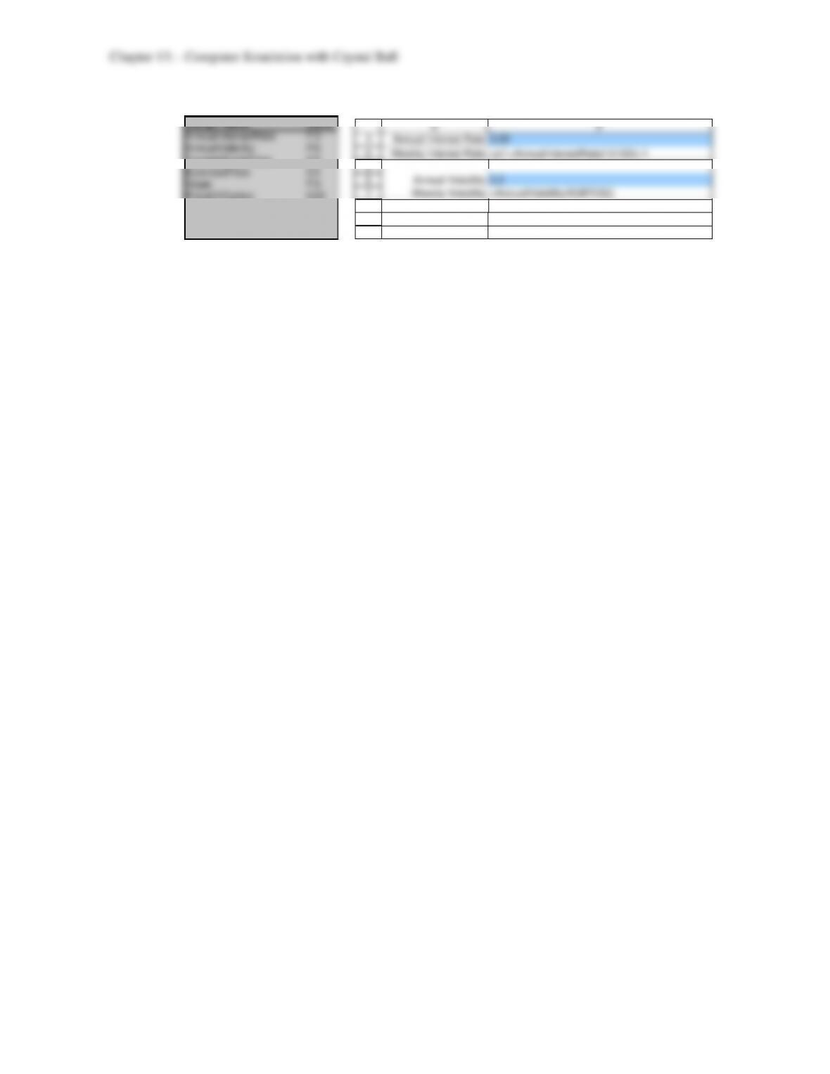
Range Name Cells
AnnualInterestRate F3
AnnualVolatility F6
CurrentStockPrice C3
ExercisePrice C4
Mean F9
PriceO fO ption C22
StandardDeviation F10
WeeklyInterestRate F4
WeeklyVolatility F7
3
4
5
6
7
8
9
10
E F
Annual Interest Rate 0.08
Weekly Interest Rate =((1+AnnualInterestRate)^(1/52))-1
Annual Volatility 0.3
Weekly Volatility =AnnualVolatility/SQRT(52)
m = =WeeklyInterestRate-0.5*(WeeklyVolatility^2)
s = =WeeklyVolatility
13–50
13–51
13–52
13–53
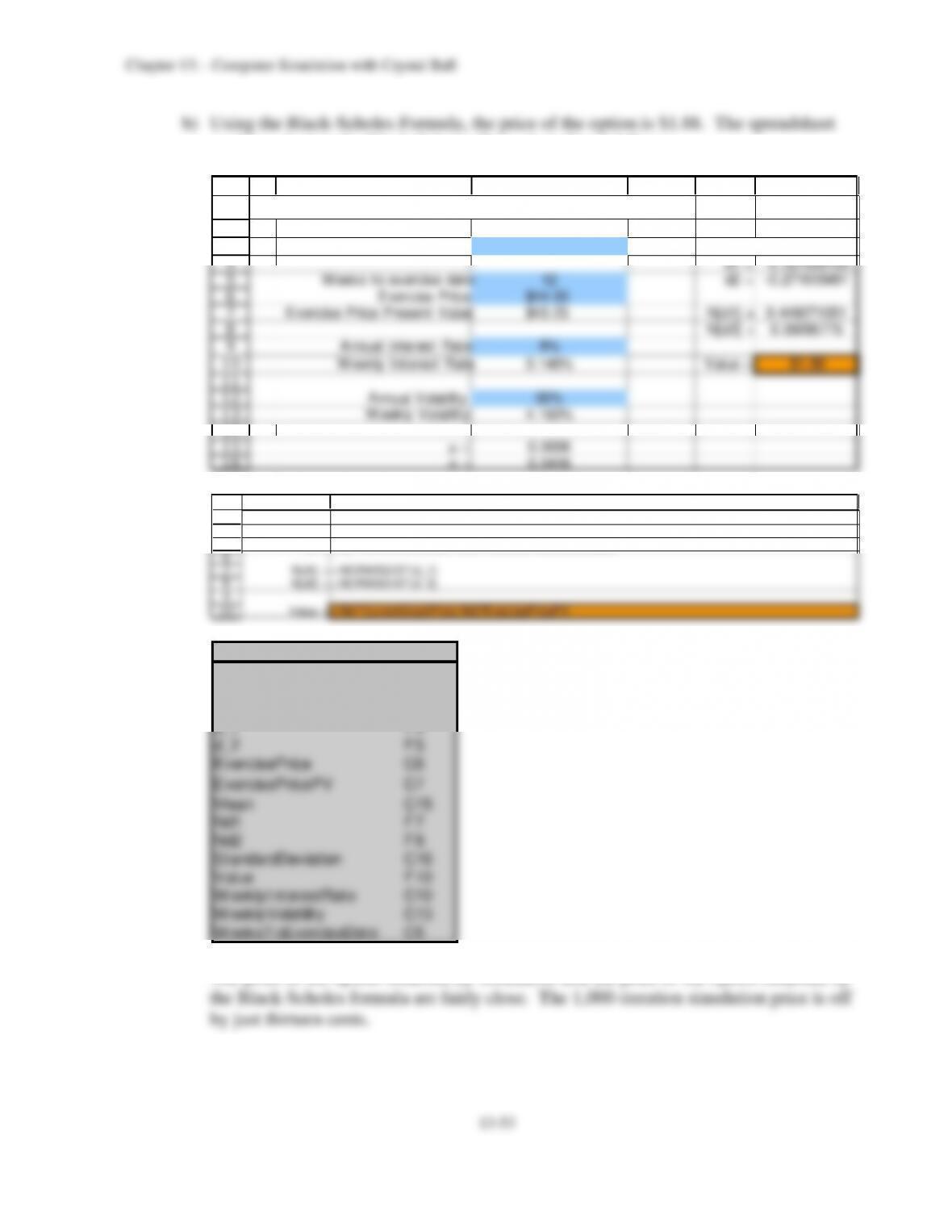
used to calculate the Black-Scholes Formula in Excel follows:
1
2
3
4
5
6
7
8
9
10
11
12
13
14
15
16
A B C D E F
Black–Scholes Calculation of Option Value
Current Stock Price $42.00 Black-Scho les
d1 = -0.127503153
W eeks to exercise date 12 d2 = -0.271618491
Exercise Price $44.00
Exercise Price Present Value $43.23 N[d1] = 0.449271051
N[d2] = 0.39295775
Annual Interest Rate 8%
W eekly Interest Rate 0.148% Value = $1.88
Annual Volatility 30%
W eekly Volatility 4.160%
= 0.0006
= 0.0416
3
4
5
6
7
8
9
10
E F
Black-Scholes
d1 =
= LN(CurrentSt ockPrice/ExercisePricePV)/ (StandardDeviation*SQ RT(W eeksT oExerciseDate))+ St andard
d2 = =d_1-StandardDeviation*SQ RT(W eeksToExerciseDate)
N[d1] = = NORMSDIST (d_1)
N[d2] = = NORMSDIST (d_2)
Value = =Nd1*CurrentStockPrice-Nd2*ExercisePricePV
Ran ge Name Cells
AnnualInterestRate C9
AnnualVolatility C12
CurrentStockPrice C3
d_1 F4
d_2 F5
ExercisePrice C6
ExercisePricePV C7
Mean C15
Nd1 F7
Nd2 F8
StandardDeviation C16
Value F10
WeeklyInterestRate C10
WeeklyVolatility C13
WeeksToExerciseDate C5
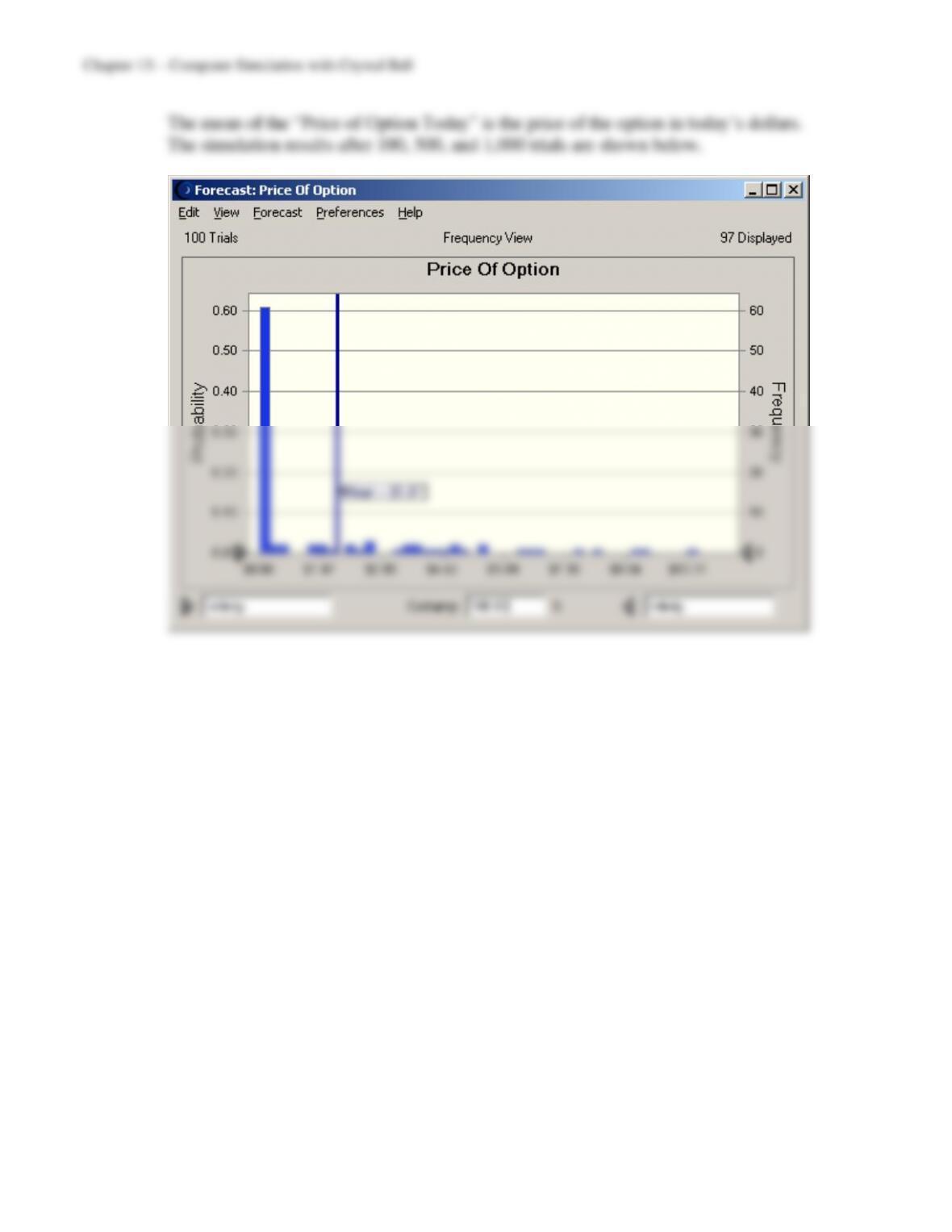
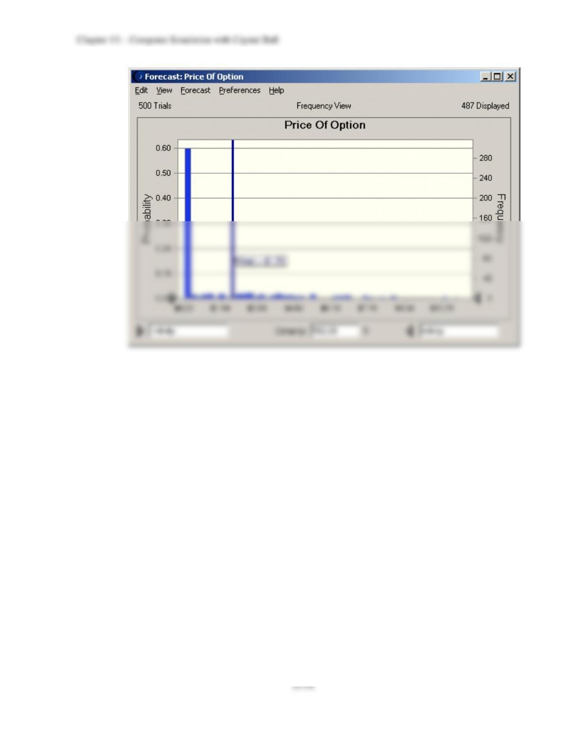
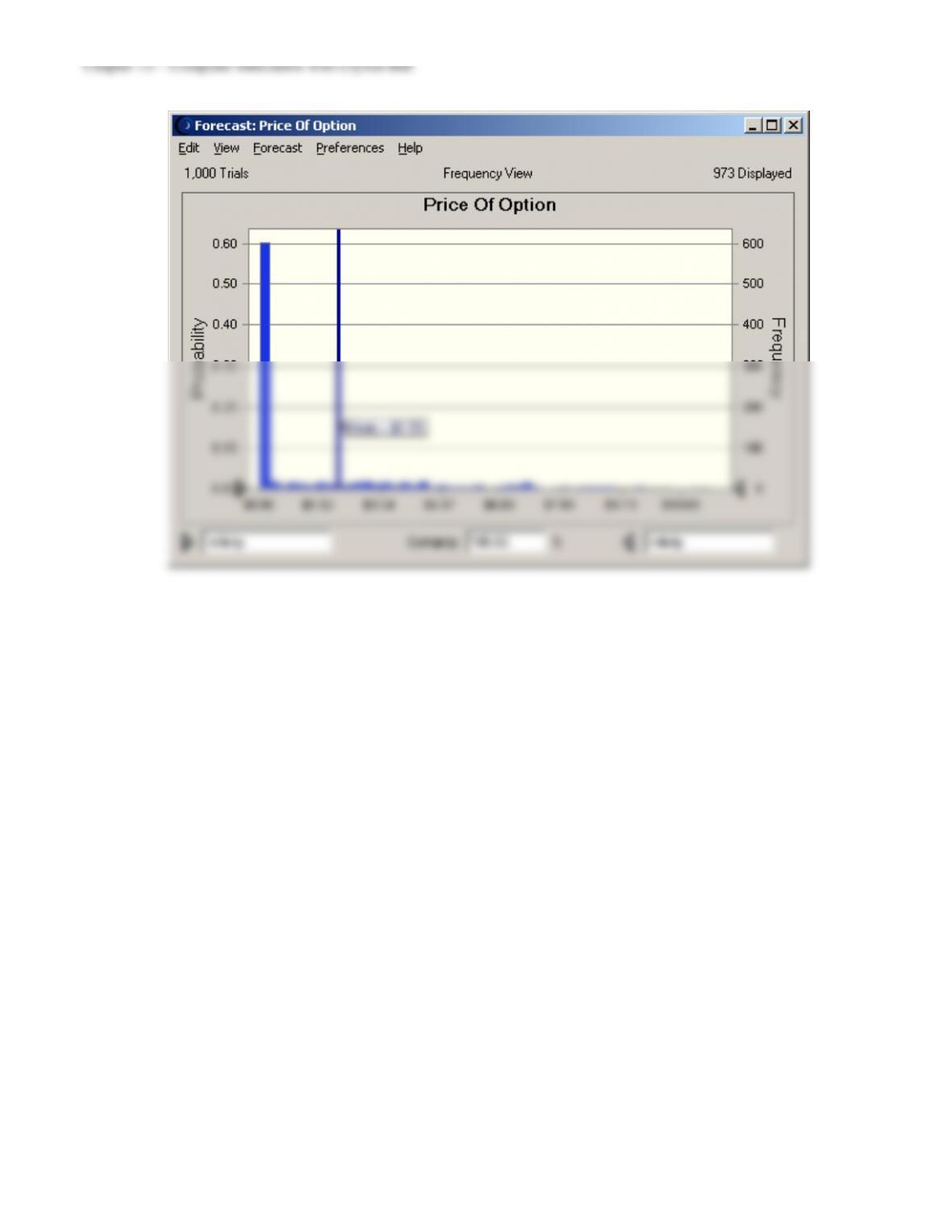
The price of the option obtained by simulation and the price of the option obtained by
13–54
c) No, a random walk does not completely describe the price movement of the stock
because the random walk assumes a consistent lognormal increase or decrease in the
price of the stock. The price of the stock could change according to a different