13-1
Chapter 13 Computer Simulation with Crystal Ball
Review Questions
13.1-1 Freddie needs to determine how many copies of the Financial Journal to order per day
from the distributor.
13.1-2 An assumption cell is a random input cell.
13.1-3 The assumed probability distribution for demand (Uniform between 40 and 70).
13.1-5 An equation for profit is entered in the forecast cell in Freddie’s spreadsheet model.
13.1-7 The key statistics provided by the statistics table are mean, median, mode, standard
deviation, and range.
13.1-9 By specifying a desired precision in the define forecast dialogue box, the simulation run
will stop when the desired precision is reached.
13.2-1 The project is to construct a new plant for a major manufacturer.
13.2-2 The three other bids are estimated in the form of a probability distribution.
13.2-5 The two possible outcomes are a loss (–$0.05 million) if the bid loses, or a profit ($0.8
million) if the bid wins.
13.3-1 The construction of a new plant for a major manufacturer.
13.3-4 A most-likely estimate, an optimistic estimate, and a pessimistic estimate.
13.3-5 The parameters can be copied and pasted for the other assumption cells.
13-2
13.4-1 How to best arrange Everglade’s financing to tide the company over until its investments in
new retirement communities can start to pay off.
13.4-3 The simulation model accounts for the great uncertainty regarding future cash flows.
13.4-4 The cash flows are the assumption cells.
13.4-5 The short-term loans are taken in a sufficiently large quantity to bring the balance up to
$0.5 million.
13.4-7 Less than 12 percent of the trials resulted in a negative cash balance at the end.
13.4-8 To take a more cautious approach in moving forward with its current plans to build more
13.5-1 A risk profile is a frequency distribution of the return from the investment.
13.5-3 The uncertainty in the cash flows for each project over the next seven years need to be
estimated.
13.5-4 The cash flows of the two projects are the assumption cells.
13.6-1 Revenue management refers to the various ways of increasing the flow of revenues through
such devices as setting up different fare classes for different categories of customers.
13.6-3 They must determine the number of reservations to accept for this flight.
13.6-5 The decision variable is the number of reservations to accept.
13.6-6 The profit, number of filled seats, and number denied boarding are all forecast cells.
13-3
13.6-7 The ticket demand and the number that show are assumption cells.
13.6-9 Although the results in this section suggest a policy of accepting 190 reservations would be
attractive, they do not demonstrate that this is necessarily the best option.
13.7-1 Twenty one.
13.7-3 One danger with using the normal distribution is that it can give negative values even when
such values are actually impossible.
13.7-4 The triangular distribution has parameters that are easy to estimate and allow the
distribution to be assymetric.
13.7-7 The three or four parameters provide great flexibility in adjusting the shape of the curve to
fit the situation.
13.7-9 The custom distribution enables you to custom-design your own probability distribution to
fit almost any unique situation you might encounter.
13.8-1 The Decision Table tool allows you to systematically apply computer simulation to identify
at least an approximation of an optimal solution.
13.8-3 Two.
13.8-4 The Step 1 dialogue box is used to choose one of the forecast cells to be the target cell.
13.8-7 The Step 3 dialogue box is used to specify the options for the Decision Table.
13.8-8 The Overlay Chart shows the results of two or more simulation runs together.
13-4
13.8-10 You can refine the analysis by generating another Decision Table with smaller intervals
13.9-1 OptQuest automatically searches for an optimal solution.
13.9-2 OptQuest can optimize problems with more than two decision variables, while a Decision
Table cannot.
13.9-3 No.
13.9-5 The Objectives pane lets you specify the objective.
13.9-7 The Constraints pane allows you to specify your constraints (if any).
13.9-8 The Options pane allows you to specify the running time.
13.9-10 If the graph remains flat for many simulations, it is reasonable to terminate the run
manually.
13.9-11 The decision variables for the project selection example needed to be binary.
Problems
13.1 a) Answers will vary. A typical set of 5 runs: $46.10, $45.38, $46.80, $45.90, $47.16.
c) The mean completion times in part b should be more consistent.
13.4 a) Uniform Distribution (Min = 299.27, Max = 498.73).
13.5
1
2
3
4
5
6
7
8
9
10
11
12
13
A B C D E F G H I J K
Now Year 1 Year 2 Year 3 Year 4 Year 5
Land Purchase Fixed -1
Construction Cost Triangular(min,likely,max) -2.4 -2 -1.6 -2
Operating Profit Normal(mean,s.dev.) 0.7 0.7 0.7 0.7 0.7 0.7
Selling Price Uniform(min,max) 4 8 6
Total Cash Flow -1 -2 0.7 0.7 0.7 6.7
Discount Factor 10%
Net Present Value ($million) 2.925
Minimum Annual Operating Profit ($million in y2-y5) 0.700
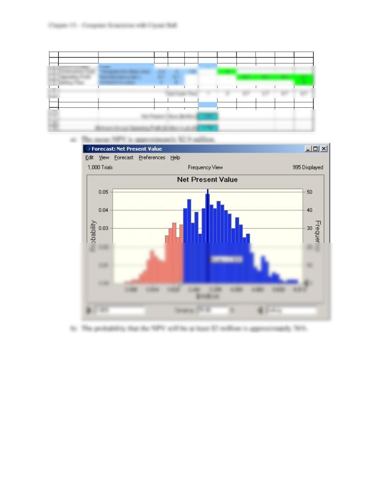
a) The mean NPV is approximately $2.9 million.
b) The probability that the NPV will be at least $2 million is approximately 76%.
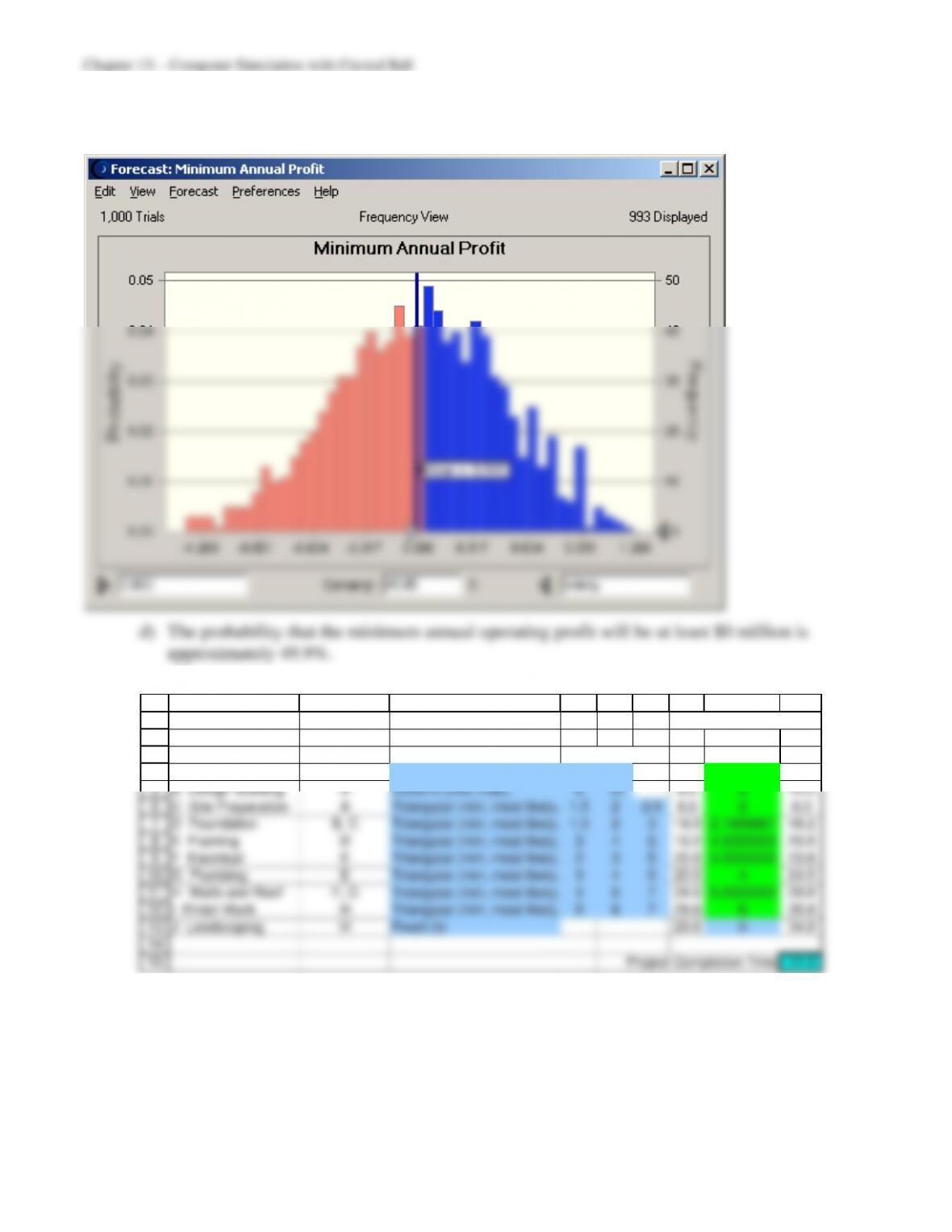
c) The mean value of the minimum annual operating profit is approximately $0
million.
13.6
1
2
3
4
5
6
7
8
9
10
11
12
13
14
15
A B C D E F G H I
(all times in months)
Start Activity Finish
Activity Predecessor Distribution Parameters Time Time Time
A Secure funding —Normal (mean, st. dev.) 6 1 0.0 6 6.0
B Design Building A Uniform (min, max) 6 10 6.0 8 14.0
C Site Preparation A
Triangular (min, most likely,
1.5 2 2.5 6.0 2 8.0
D Foundation B, C
Triangular (min, most likely,
1.5 2 3 14.0 2.1666667 16.2
E Framing D
Triangular (min, most likely,
3 4 6 16.2 4.3333333 20.5
F Electrical E
Triangular (min, most likely,
2 3 5 20.5 3.3333333 23.8
G Plumbing E
Triangular (min, most likely,
3 4 5 20.5 4 24.5
H Walls and Roof F, G
Triangular (min, most likely,
4 5 7 24.5 5.3333333 29.8
I Finish Work H
Triangular (min, most likely,
5 6 7 29.8 6 35.8
J Landscaping H Fixed (5) 29.8 5 34.8
Project Completion Time 34.8
13-7
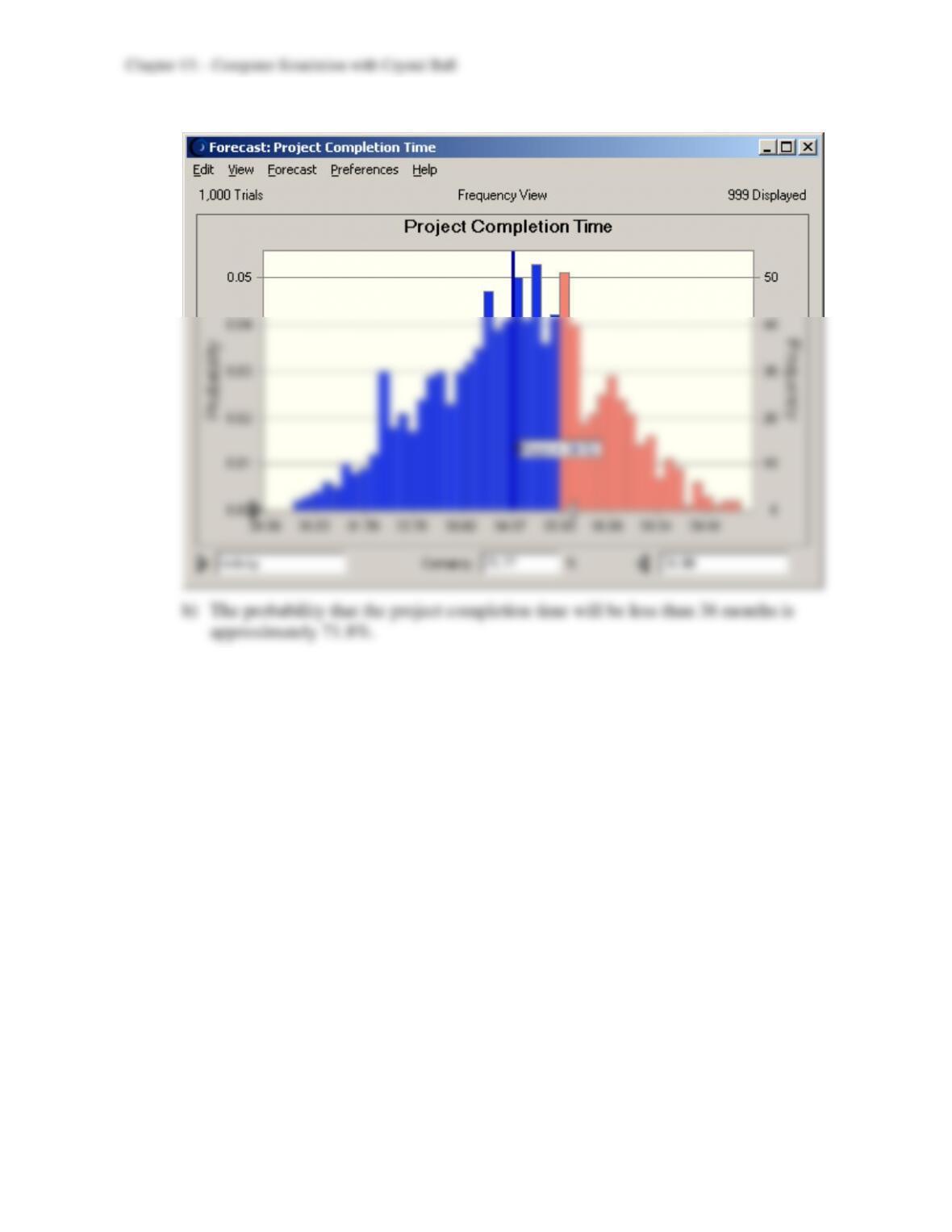
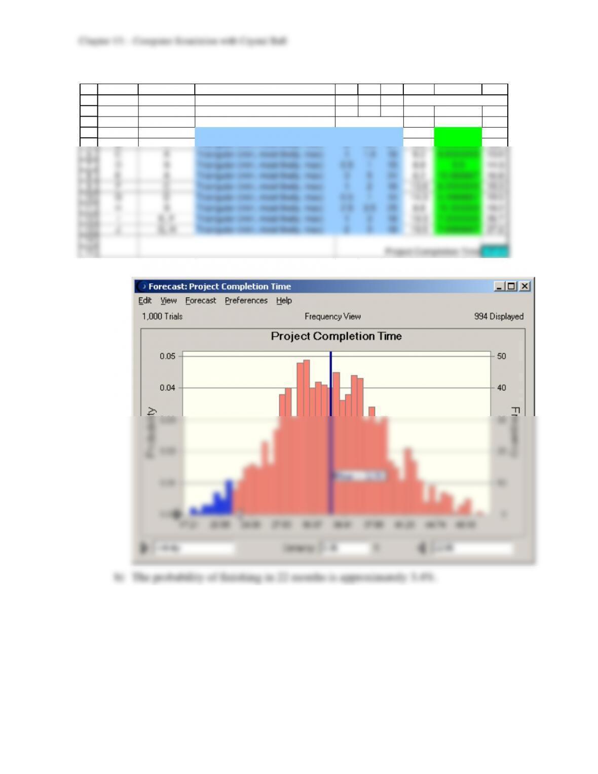
a) The mean project completion time is approximately 35 months.
13-8
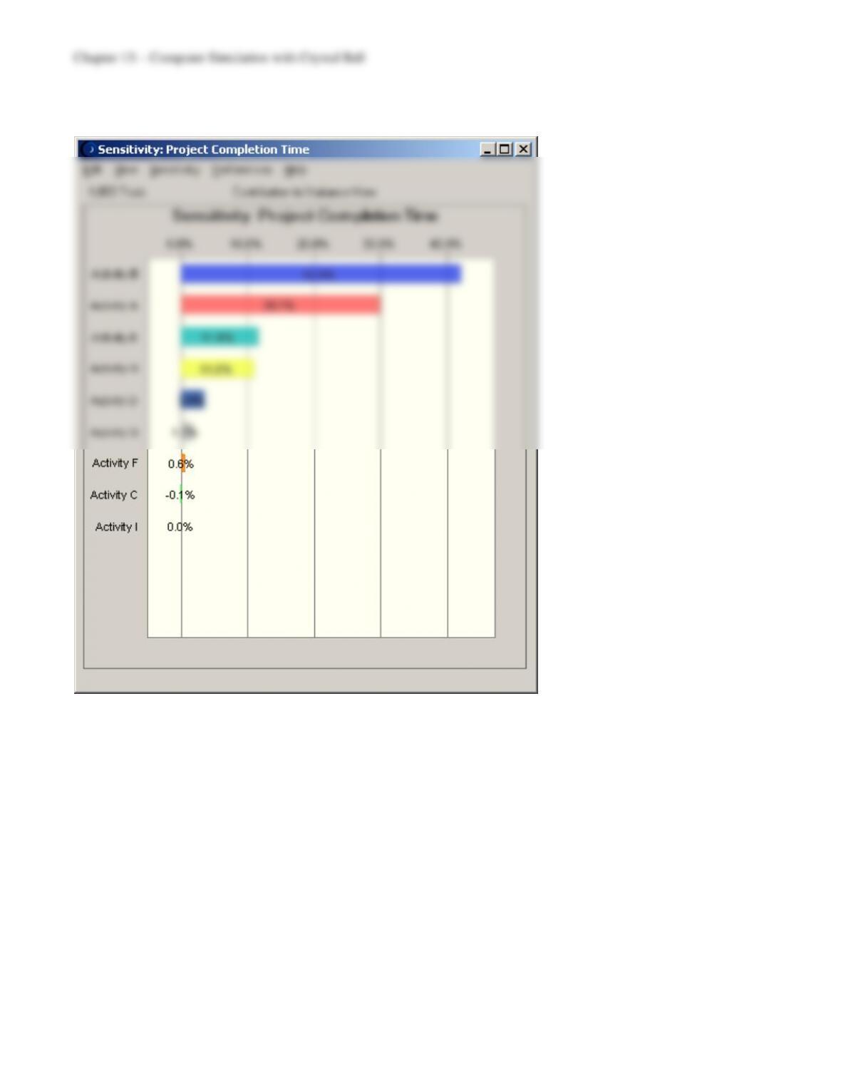
c) Activity B and then Activity A have the largest impact on the variability of the
project completion time.
13.7
1
2
3
4
5
6
7
8
9
10
11
12
13
14
15
A B C D E F G H I
(all times in months)
Start Activity Finish
Activity Predecessor Distribution Parameters Time Time Time
A—Triangular (min, most likely, max) 1.5 2 15 0.0 6.1666667 6.2
B—Triangular (min, most likely, max) 2 3.5 21 0.0 8.8333333 8.8
C A Triangular (min, most likely, max) 1 1.5 18 6.2 6.8333333 13.0
D B Triangular (min, most likely, max) 0.5 1 15 8.8 5.5 14.3
E A Triangular (min, most likely, max) 3 5 24 6.2 10.666667 16.8
F C Triangular (min, most likely, max) 1 2 16 13.0 6.3333333 19.3
G D Triangular (min, most likely, max) 0.5 1 14 14.3 5.1666667 19.5
H B Triangular (min, most likely, max) 2.5 3.5 25 8.8 10.333333 19.2
IE, F Triangular (min, most likely, max) 1 3 18 19.3 7.3333333 26.7
J G, H Triangular (min, most likely, max) 2 3 18 19.5 7.6666667 27.2
Project Completion Time 27.2
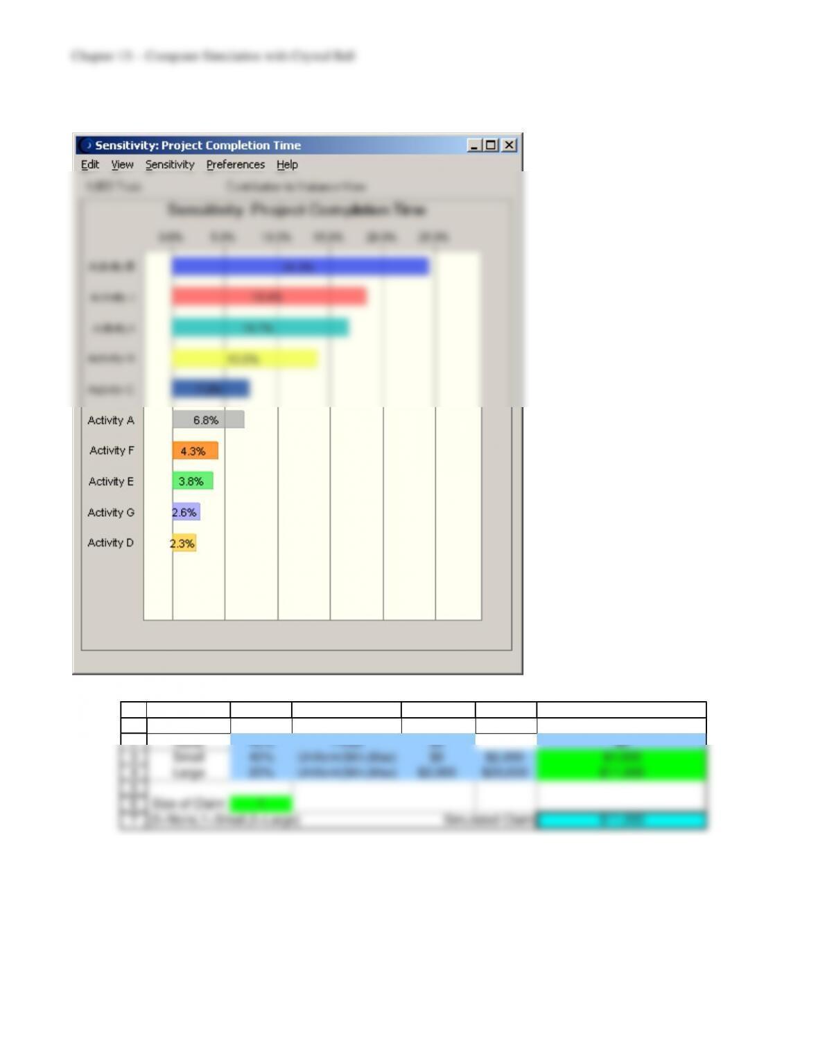
a) The mean project completion time is approximately 33 months.
13–10
c) Activities B and J have the largest impact on the variability of the project
completion time.
13.8
1
2
3
4
5
6
7
A B C D E F
Size of Claim Prob. Distribution Parameters Claim (If Claim is This Size)
None 40% Fixed $0 $0
Small 40% Uniform(Min,Max) $0 $2,000 $1,000
Large 20% Uniform(Min,Max) $2,000 $20,000 $11,000
Size of Claim 1
(0=None,1=Small,2=Large) Simulated Claim $11,000
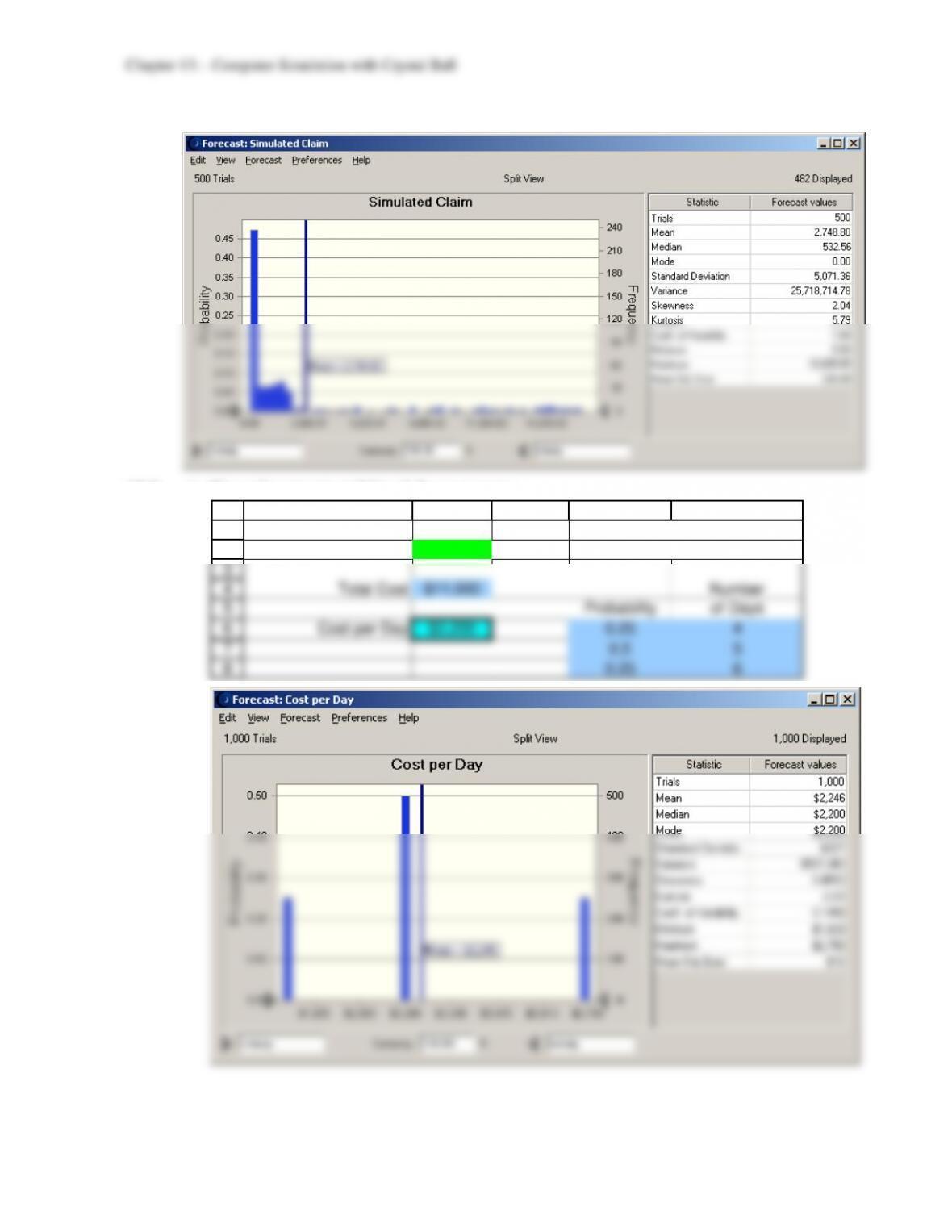
The mean claim is approximately $2,750.
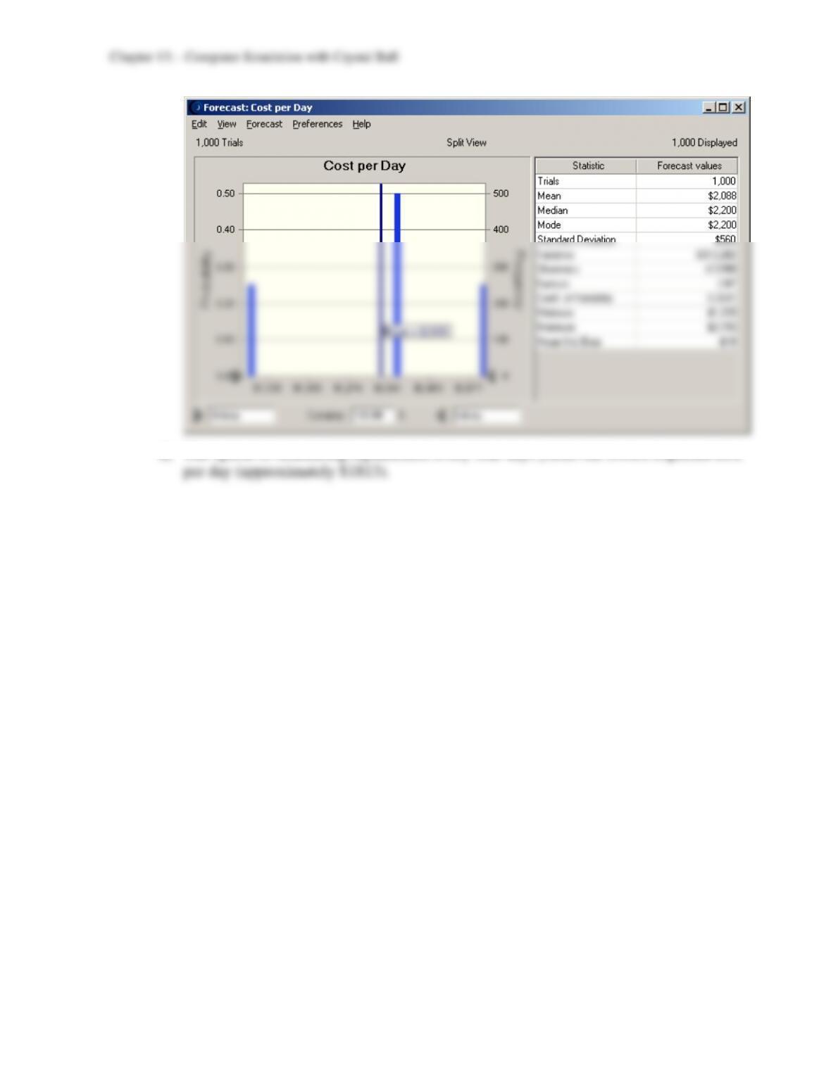
13.9 a) No replacement until breakdown occurs:
1
2
3
4
5
6
7
8
A B C D E
Distribution of
Days Until Breakdown 5
Time between Breakdowns
Total Cost $11,000 Number
Probability of Days
Cost per Day $2,200 0.25 4
0.5 5
0.25 6
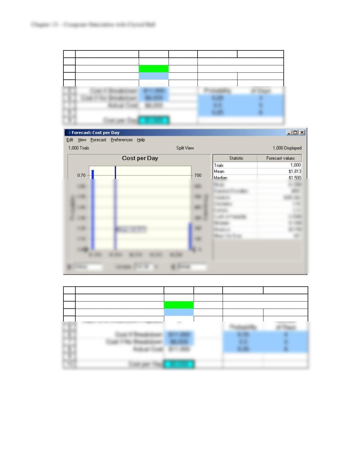
b) Scheduled replacement after 4 days:
1
2
3
4
5
6
7
8
9
A B C D E
Distribution of
Days Until Breakdown 5
Time between Breakdowns
Days Until Replace 4
Number
Cost if Breakdown $11,000 Probability of Days
Cost if No Breakdown $6,000 0.25 4
Actual Cost $6,000 0.5 5
0.25 6
Cost per Day $1,500
c) Scheduled replacement after 5 days:
1
2
3
4
5
6
7
8
9
10
A B C D E
Distribution of
Days Until Breakdown 5
Time between Breakdowns
Days Until Replace 5
Days Until Breakdown/Replace 5 Number
Probability of Days
Cost if Breakdown $11,000 0.25 4
Cost if No Breakdown $6,000 0.5 5
Actual Cost $11,000 0.25 6
Cost per Day $2,200
13–13
d) The option of scheduling replacement every four days yields the lowest expected cost
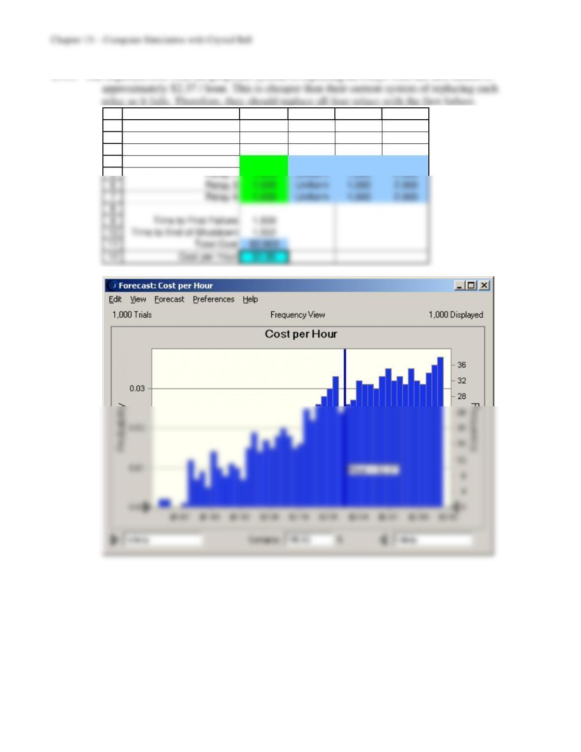
13.10 The expected cost with the proposed system of replacing all relays with the first failure is
1
2
3
4
5
6
7
8
9
10
11
12
A B C D E
Time to
Failure
(hours) Min Max
Relay 1 1,500 Uniform 1,000 2,000
Relay 2 1,500 Uniform 1,000 2,000
Relay 3 1,500 Uniform 1,000 2,000
Relay 4 1,500 Uniform 1,000 2,000
Time to First Failure 1,500
Time to End of Shutdown 1,502
Total Cost $2,800
Cost per Hour $1.86
13–15
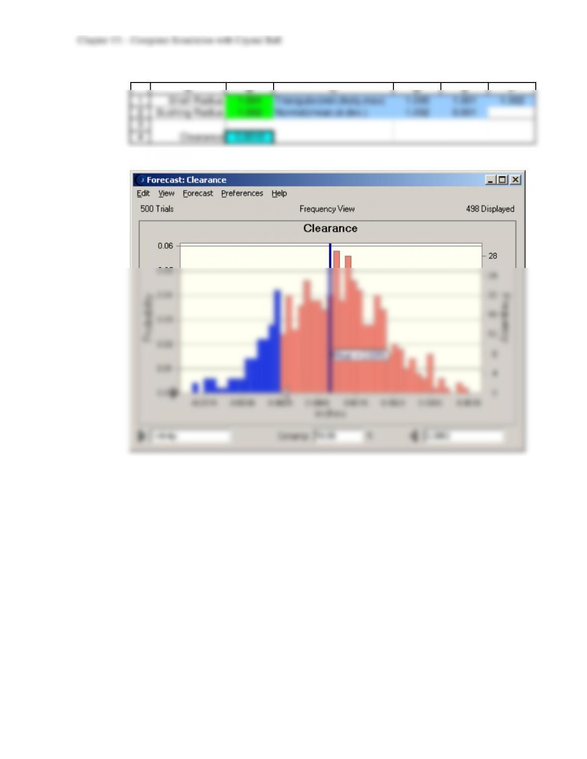
13.11 There is an approximately 18.1% chance of negative clearance.
1
2
3
4
A B C D E F
Shaft Radius 1.001 Triangular(min,likely,max) 1.000 1.001 1.002
Bushing Radius 1.002 Normal(mean,st.dev.) 1.002 0.001
Clearance 0.0010
13–16
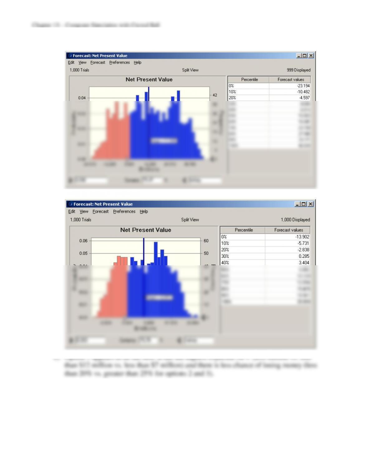
13.12 a) Option 2 (Hotel Project only):
b) Option 3 (Shopping Center Project only):
13.13
1
2
3
4
5
6
7
8
9
10
11
12
13
14
15
16
17
18
19
20
21
22
23
24
25
26
27
28
29
30
31
A B C D E F G H I
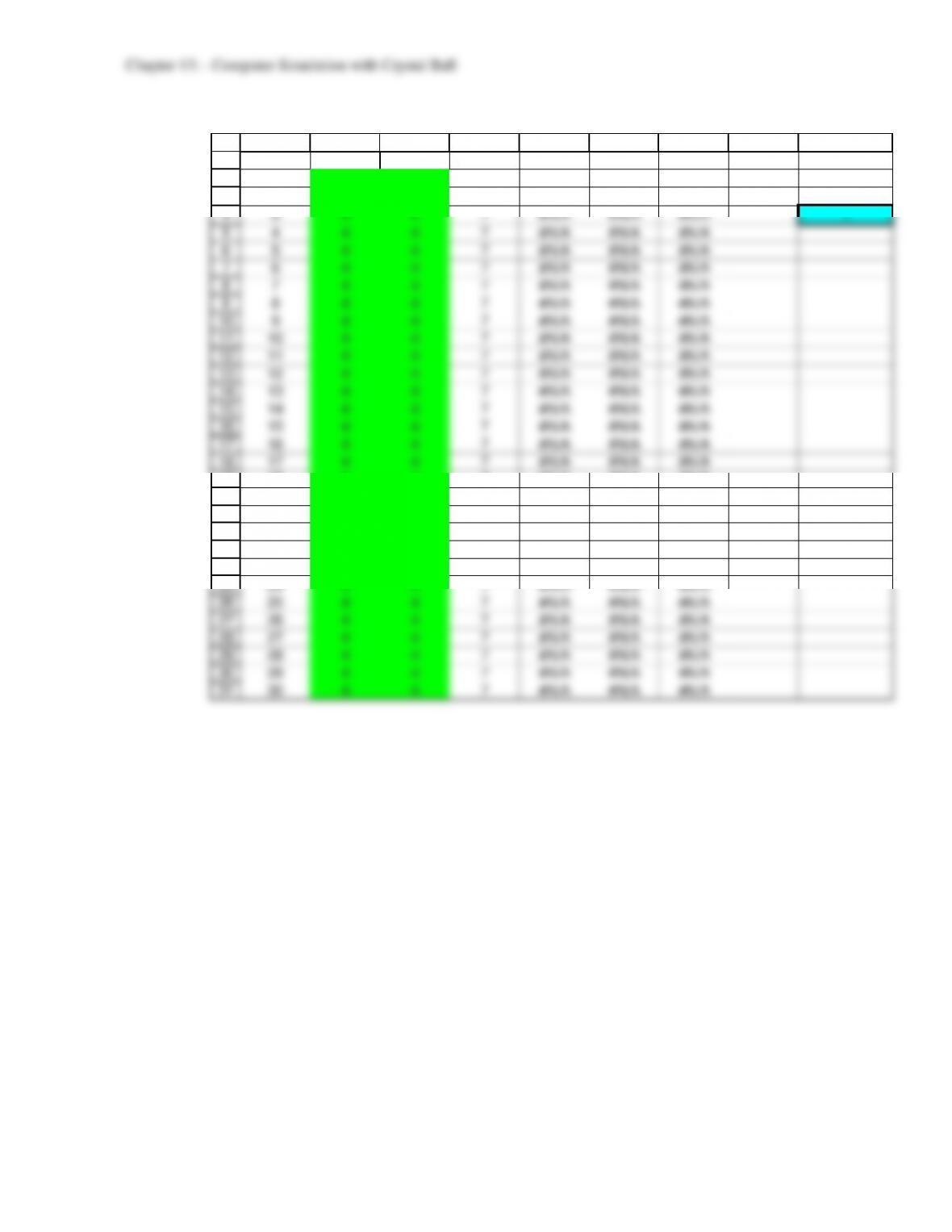
Toss Die 1 Die 2 Sum Win? Lose? Continue? Win
1 4 4 7 Yes No No Game?
2 4 4 7 #N/A #N/A #N/A (1=yes,0=no)
3 4 4 7 #N/A #N/A #N/A 1
4 4 4 7 #N/A #N/A #N/A
5 4 4 7 #N/A #N/A #N/A
6 4 4 7 #N/A #N/A #N/A
7 4 4 7 #N/A #N/A #N/A
8 4 4 7 #N/A #N/A #N/A
9 4 4 7 #N/A #N/A #N/A
10 4 4 7 #N/A #N/A #N/A
11 4 4 7 #N/A #N/A #N/A
12 4 4 7 #N/A #N/A #N/A
13 4 4 7 #N/A #N/A #N/A
14 4 4 7 #N/A #N/A #N/A
15 4 4 7 #N/A #N/A #N/A
16 4 4 7 #N/A #N/A #N/A
17 4 4 7 #N/A #N/A #N/A
18 4 4 7 #N/A #N/A #N/A
19 4 4 7 #N/A #N/A #N/A
20 4 4 7 #N/A #N/A #N/A
21 4 4 7 #N/A #N/A #N/A
22 4 4 7 #N/A #N/A #N/A
23 4 4 7 #N/A #N/A #N/A
24 4 4 7 #N/A #N/A #N/A
25 4 4 7 #N/A #N/A #N/A
26 4 4 7 #N/A #N/A #N/A
27 4 4 7 #N/A #N/A #N/A
28 4 4 7 #N/A #N/A #N/A
29 4 4 7 #N/A #N/A #N/A
30 4 4 7 #N/A #N/A #N/A
13–18
13–19
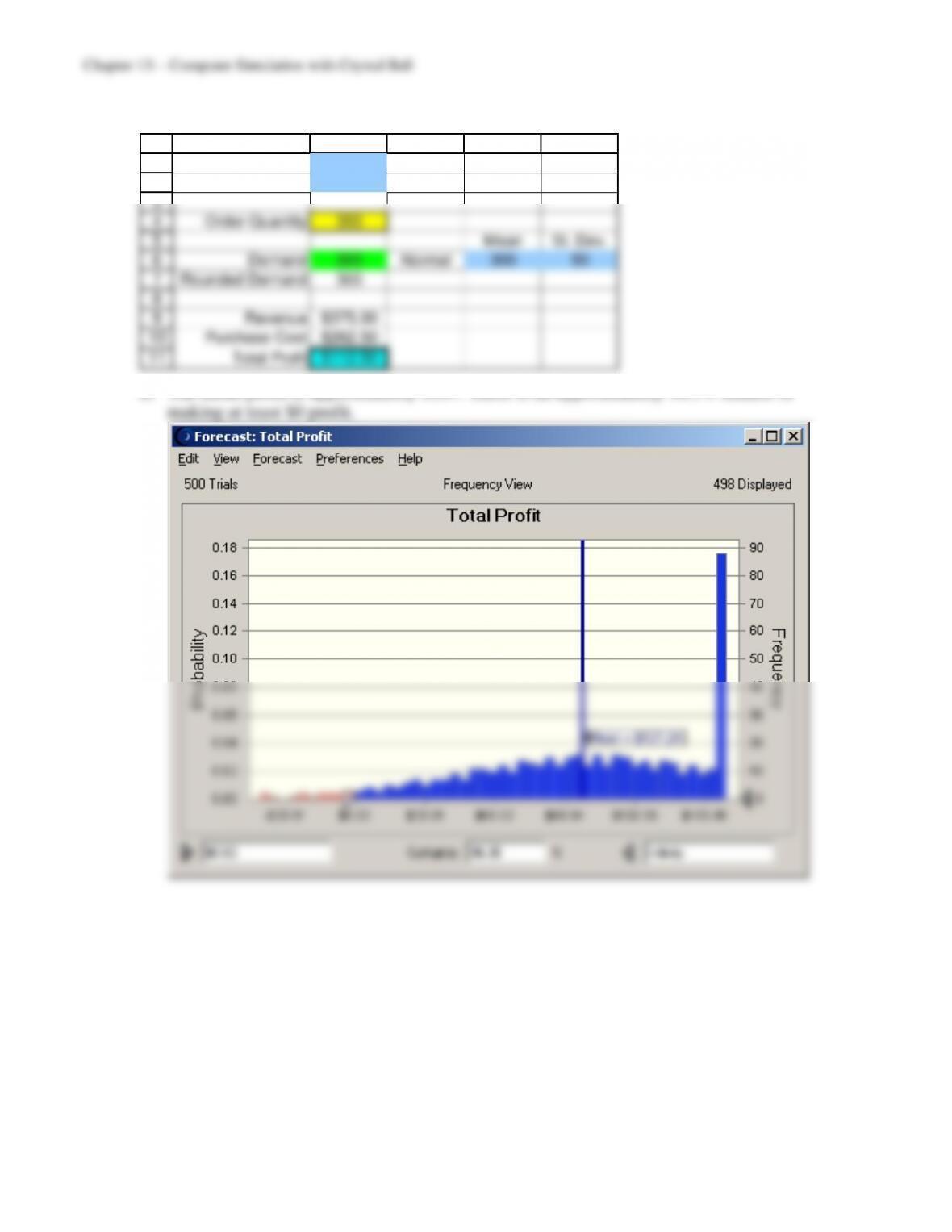
13.14 The order quantity that maximizes the mean profit is approximately 55.
Order Quantity (50)
Order Quantity (51)
Order Quantity (52)
Order Quantity (53)
Order Quantity (54)
Order Quantity (55)
Order Quantity (56)
Order Quantity (57)
Order Quantity (58)
Order Quantity (59)
Order Quantity (60)
$46.67 $46.97 $47.20 $47.36 $47.46 $47.50 $47.46 $47.36 $47.20 $46.96 $46.66
13.15
1
2
3
4
5
6
7
8
9
10
11
A B C D E
Purchase Price $0.75
Selling Price $1.25
Order Quantity 350
Mean St. Dev.
Demand 300 Normal 300 50
Rounded Demand 300
Revenue $375.00
Purchase Cost $262.50
Total Profit $112.50
a) The mean profit is approximately $107. There is an approximately 96.3% chance of