12–18
12.16 a) Two tellers:
1
2
3
4
5
6
7
8
9
10
11
12
13
14
15
16
17
18
19
20
21
A B C D E F G H
Template for Queueing Simulation
Data Results
Number of Servers = 2 Point
Estimate Low High
Interarrival Times L = 1.78757206 1.726441349 1.848702773
Distribution = Translated Exponential Lq = 0.28220656 0.241680028 0.322733085
Minimum Value = 0.5 W = 1.79878512 1.747588762 1.84998147
Mean = 1 Wq = 0.28397678 0.244772435 0.32318112
Service T imes P0 = 0.07738102 0.069798855 0.084963186
Distribution = Erlang P1 = 0.33987245 0.324592313 0.355152593
Mean = 1.5 P2 = 0.37038029 0.359243093 0.381517479
k = 4 P3 = 0.15923981 0.147308796 0.171170825
P4 = 0.0402521 0.032237042 0.048267158
Length of Simu lation Run P5 = 0.00942833 0.005068991 0.01378767
Number of Arrivals = 5,000 P6 = 0.00305244 0.000233056 0.005871825
P7
=0.00039356 -0.000134342 0.00092146
P8 = 0 0 0
P9 = 0 0 0
P10 = 0 0 0
95% Confidence Interval
Run Simulation
b) Three tellers:
1
2
3
4
5
6
7
8
9
10
11
12
13
14
15
16
17
18
19
20
21
A B C D E F G H
Template for Queueing Simulation
Data Results
Number of Servers = 3 Point
Estimate Low High
Interarrival Times L = 1.50460097 1.471382686 1.537819251
Distribution = Translated Exponential Lq = 0.0143989 0.010570703 0.018227099
Minimum Value = 0.5 W = 1.51807552 1.495626801 1.540524241
Mean = 1 Wq = 0.01452785 0.010727933 0.018327771
Service T imes P0 = 0.11217696 0.103577706 0.120776216
Distribution = Erlang P1 = 0.40463781 0.392449367 0.416826253
Mean = 1.5 P2 = 0.36399143 0.353062436 0.374920422
k = 4 P3 = 0.10560031 0.097335384 0.11386524
P4 = 0.01278807 0.009713729 0.015862418
Length of Simu lation Run P5 = 0.00080541 0.000273786 0.001337042
Number of Arrivals = 5,000 P6 = 0 0 0
P7
=0 0 0
P8 = 0 0 0
P9 = 0 0 0
P10 = 0 0 0
95% Confidence Interval
Run Simulation
12–19
c) Two Tellers:
1
2
3
4
5
6
7
8
9
10
11
12
13
14
15
16
17
18
19
20
21
A B C D E F G H
Template for Queueing Simulation
Data Results
Number of Servers = 2 Point
Estimate Low High
Interarrival Times L = 2.28526178 2.151379363 2.41914419
Distribution = Translated Exponential Lq = 0.62386582 0.509969808 0.737761839
Minimum Value = 0.5 W = 2.06648116 1.955490349 2.17747197
Mean = 0.9 Wq = 0.56413973 0.463906706 0.664372761
Service T imes P0 = 0.04566936 0.039854091 0.051484635
Distribution = Erlang P1 = 0.24726532 0.228502346 0.266028296
Mean = 1.5 P2 = 0.34164446 0.322145294 0.361143622
k = 4 P3 = 0.20698293 0.191836287 0.222129571
P4 = 0.09262055 0.078093733 0.107147361
Length of Simu lation Run P5 = 0.04326281 0.028218881 0.05830673
Number of Arrivals = 5,000 P6 = 0.01491818 0.007216274 0.022620095
P7
=0.00493725 0.00059847 0.009276032
P8 = 0.00176965 -0.000692721 0.004232024
P9 = 0.00055943 -0.000522109 0.001640977
P10 = 0.00037006 -0.000345366 0.001085478
95% Confidence Interval
Run Simulation
Three Tellers:
1
2
3
4
5
6
7
8
9
10
11
12
13
14
15
16
17
18
19
20
21
A B C D E F G H
Template for Queueing Simulation
Data Results
Number of Servers = 3 Point
Estimate Low High
Interarrival Times L = 1.65729454 1.622102655 1.692486433
Distribution = Translated Exponential Lq = 0.02092004 0.015617543 0.02622253
Minimum Value = 0.5 W = 1.50026698 1.47758434 1.522949616
Mean = 0.9 Wq = 0.01893788 0.014214235 0.023661518
Service T imes P0 = 0.07593852 0.068988925 0.082888121
Distribution = Erlang P1 = 0.36784219 0.35533123 0.380353149
Mean = 1.5 P2 = 0.40012554 0.389988281 0.410262808
k = 4 P3 = 0.13649752 0.127031262 0.145963775
P4 = 0.01840906 0.014574934 0.022243189
Length of Simu lation Run P5 = 0.00105051 0.000226165 0.001874863
Number of Arrivals = 5,000 P6 = 0.00013665 -0.000130284 0.000403582
P7
=0 0 0
P8 = 0 0 0
P9 = 0 0 0
P10 = 0 0 0
95% Confidence Interval
Run Simulation
d) Two tellers provides reasonable wait times, with both the original arrival rate (Wq = 0.3
minutes) and the higher arrival rate in part c (Wq = 0.6 minutes).
12.17 a&b) German cars:
1
2
3
4
5
6
7
8
9
10
11
12
13
14
107
108
109
A B C D E F G H
Mean Interarrival Time = 0.25 days
Mean Service Time = 0.2 days
Average Time in Line (W q) = 0.54 days
Average Time in System (W) = 0.72 days
Time Time Time Time Time
Customer Interarrival of Service Service Service in in
Arrival Time Arrival Begins Time Ends Line System
1 0.36 0.36 0.36 0.15 0.51 0.00 0.15
2 0.15 0.50 0.51 0.09 0.59 0.00 0.09
3 0.17 0.68 0.68 0.05 0.72 0.00 0.05
4 0.05 0.73 0.73 0.00 0.73 0.00 0.00
5 0.11 0.83 0.83 0.03 0.87 0.00 0.03
98 0.03 21.35 21.67 0.53 22.21 0.33 0.86
99 0.15 21.49 22.21 0.20 22.40 0.71 0.91
100 0.42 21.91 22.40 0.18 22.59 0.49 0.68
12–20
c) Japanese Cars:
1
2
3
4
5
6
7
8
9
10
11
12
13
14
107
108
109
A B C D E F G H
Mean Interarrival Time = 0.5 days
Mean Service Time = 0.2 days
Average Time in Line (W q) = 0.19 days
Average Time in System (W) = 0.38 days
Time Time Time Time T ime
Customer Interarrival of Service Service Service in in
Arrival Time Arrival Begins Time Ends Line System
1 1.11 1.11 1.11 0.17 1.28 0.00 0.17
2 0.16 1.27 1.28 0.12 1.40 0.01 0.13
3 0.52 1.79 1.79 0.31 2.11 0.00 0.31
4 0.39 2.18 2.18 0.07 2.25 0.00 0.07
5 0.15 2.34 2.34 0.31 2.64 0.00 0.31
98 0.34 41.26 41.26 0.09 41.35 0.00 0.09
99 0.05 41.31 41.35 0.06 41.42 0.04 0.10
100 0.50 41.81 41.81 0.25 42.06 0.00 0.25
d) German cars:
1
2
3
4
5
6
7
8
9
10
11
12
13
14
15
16
17
18
19
20
21
A B C D E F G H
Template for Queueing Simulation
Data Results
Number of Servers = 1 Point
Estimate Low High
Interarrival Times L = 4.87903777 3.344529192 6.413546353
Distribution = Exponential Lq = 4.06903737 2.552881224 5.585193514
Mean = 0.25 W = 1.21741101 0.84623223 1.588589799
0.9 Wq = 1.01530079 0.646688099 1.383913484
Service T imes P0 = 0.1899996 0.16425264 0.215746552
Distribution = Exponential P1 = 0.15101797 0.132489844 0.169546091
Mean = 0.2 P2 = 0.12530975 0.111337121 0.139282371
4P3 = 0.09541037 0.084720833 0.106099913
P4 = 0.07620596 0.066901918 0.085509995
Length of Simu lation Run P5 = 0.06224509 0.054038618 0.070451571
Number of Arrivals = 10,000 P6 = 0.05620591 0.047527927 0.064883901
P7
=0.0420322 0.035157883 0.048906526
P8 = 0.03118735 0.025046424 0.037328273
P9 = 0.02715091 0.020825618 0.033476206
P10 = 0.02295245 0.016668188 0.029236719
95% Confidence Interval
Run Simulation
Japanese cars:
1
2
3
4
5
6
7
8
9
10
11
12
13
14
15
16
17
18
19
20
21
A B C D E F G H
Template for Queueing Simulation
Data Results
Number of Servers = 1 Point
Estimate Low High
Interarrival Times L = 0.65120353 0.616465588 0.685941467
Distribution = Exponential Lq = 0.2558739 0.229868433 0.281879358
Mean = 0.5 W = 0.32892631 0.314496732 0.343355886
0.9 Wq = 0.12924324 0.117271635 0.141214851
Service T imes P0 = 0.60467037 0.593750466 0.61559027
Distribution = Exponential P1 = 0.24147266 0.235575489 0.247369829
Mean = 0.2 P2 = 0.09287404 0.088050078 0.097697993
4P3 = 0.03700232 0.03325512 0.040749518
P4 = 0.01370641 0.011375648 0.016037177
Length of Simu lation Run P5 = 0.00584073 0.004206205 0.007475253
Number of Arrivals = 10,000 P6 = 0.00268974 0.00151472 0.00386477
P7
=0.00123847 0.000427242 0.002049696
P8 = 0.00040858 5.34782E-05 0.000763672
P9 = 9.6687E-05 -2.05314E-05 0.000213906
P10 = 0 0 0
95% Confidence Interval
Run Simulation
12–21
e)
1
2
3
4
5
6
7
8
9
10
11
12
13
14
15
16
17
18
19
20
21
A B C D E F G H
Template for Queueing Simulation
Data Results
Number of Servers = 2 Point
Estimate Low High
Interarrival Times L = 0.95366646 0.915224212 0.992108704
Distribution = Exponential Lq = 0.14883976 0.12864295 0.16903656
Mean = 0.25 W = 0.23825778 0.230627162 0.245888395
0.9 Wq = 0.03718515 0.032400866 0.041969432
Service T imes P0 = 0.42884693 0.416925848 0.440768021
Distribution = Exponential P1 = 0.33747943 0.329623104 0.345335752
Mean = 0.2 P2 = 0.14057768 0.134585017 0.14657034
4P3 = 0.05713271 0.052879164 0.061386253
P4 = 0.02275274 0.0195675 0.025937975
Length of Simu lation Run P5 = 0.00872319 0.006702754 0.010743624
Number of Arrivals = 10,000 P6 = 0.00280179 0.001657449 0.003946123
P7
=0.00130463 0.000252912 0.002356338
P8 = 0.00036465 2.98821E-05 0.000699427
P9 = 1.6258E-05 -1.19183E-05 4.44348E-05
P10 = 0 0 0
95% Confidence Interval
Run Simulation
f) This option significantly decreases the waiting time for German cars without the added
cost of an additional mechanic.
1
2
3
4
5
6
7
8
9
10
11
12
13
14
15
16
17
18
19
20
21
A B C D E F G H
Template for Queueing Simulation
Data Results
Number of Servers = 2 Point
Estimate Low High
Interarrival Times L = 2.28578801 2.159897988 2.411678029
Distribution = Exponential Lq = 0.97253541 0.865389879 1.079680942
Mean = 0.166666667 W = 0.38167957 0.362993929 0.40036522
0.9 Wq = 0.16239341 0.145460556 0.179326257
Service T imes P0 = 0.20793417 0.198318894 0.217549454
Distribution = Exponential P1 = 0.27087905 0.261765572 0.279992536
Mean = 0.22 P2 = 0.17706771 0.17137547 0.182759946
4P3 = 0.12005889 0.114963795 0.125153977
P4 = 0.08071505 0.076004425 0.085425668
Length of Simu lation Run P5 = 0.05162234 0.047503838 0.055740836
Number of Arrivals = 20,000 P6 = 0.03282908 0.029305955 0.036352202
P7
=0.01987242 0.016883839 0.022861011
P8 = 0.01363915 0.011115994 0.016162305
P9 = 0.00977922 0.007382485 0.01217596
P10 = 0.00562584 0.003894695 0.007356992
95% Confidence Interval
Run Simulation
g)
Question Part
Simulated Estimate for W
Analytical Value for W
b
0.72 days
1.00 days
c
0.38 days
0.33 days
d (German)
d (Japanese)
1.22 days
0.32 days
1.00 days
0.33 days
e
0.24 days
0.24 days
f
0.38 days
0.39 days
The results of the simulation were quite accurate for all but part b, where only 100
12–22
h) Answers will vary. The option of training the two current mechanics significantly
decreases the waiting time for German cars, without a significant impact on the wait for
12.18 a & b) Monitors:
1
2
3
4
5
6
7
8
9
10
11
12
13
14
15
108
109
110
A B C D E F G H
Minimum Interarrival Time = 10 minutes
Maximum Interarrival Time = 20 minutes
Mean Service T ime = 10 minutes
Average T ime in Line (W q) = 14.74 minutes
Average T ime in System (W ) = 25.35 minutes
Time Time Time Time Time
Customer Interarrival of Service Service Service in in
Arrival Time Arrival Begins Time Ends Line System
1 16.63 16.63 16.63 1.28 17.90 0.00 1.28
2 19.47 36.09 36.09 4.44 40.54 0.00 4.44
3 17.82 53.91 53.91 15.50 69.41 0.00 15.50
4 13.47 67.38 69.41 38.51 107.92 2.03 40.54
5 13.95 81.33 107.92 1.02 108.94 26.59 27.61
98 13.29 1495.09 1495.09 0.10 1495.19 0.00 0.10
99 17.95 1513.04 1513.04 5.27 1518.30 0.00 5.27
100 19.03 1532.06 1532.06 9.23 1541.29 0.00 9.23
c) Printers:
1
2
3
4
5
6
7
8
9
10
11
12
13
14
107
108
109
A B C D E F G H
Interarrival T ime (constant) = 15 minutes
Mean Service Time = 10 minutes
Average Time in Line (Wq) = 17.58 minutes
Average Time in System (W ) = 28.66 minutes
Time Time Time Time Time
Customer Interarrival of Service Service Service in in
Arrival Time Arrival Begins Time Ends Line System
1 15.00 15.00 15.00 6.43 21.43 0.00 6.43
2 15.00 30.00 30.00 2.11 32.11 0.00 2.11
3 15.00 45.00 45.00 3.88 48.88 0.00 3.88
4 15.00 60.00 60.00 16.73 76.73 0.00 16.73
5 15.00 75.00 76.73 13.82 90.54 1.73 15.54
98 15.00 1470.00 1470.00 5.78 1475.78 0.00 5.78
99 15.00 1485.00 1485.00 6.72 1491.72 0.00 6.72
100 15.00 1500.00 1500.00 10.55 1510.55 0.00 10.55
12–23
d) Monitors:
1
2
3
4
5
6
7
8
9
10
11
12
13
14
15
16
17
18
19
20
21
A B C D E F G H
Template for Queueing Simulation
Data Results
Number of Servers = 1 Point
Estimate Low High
Interarrival Times L = 1.13498458 1.07761665 1.192352518
Distribution = Uniform Lq = 0.46550351 0.418032717 0.512974294
Minimum Value = 10 W = 16.9947443 16.14318643 17.84630211
Maximum Value = 20 Wq = 6.97023831 6.262667949 7.677808666
Service T imes P0 = 0.33051892 0.318142623 0.342895219
Distribution = Exponential P1 = 0.38391562 0.374495424 0.39333582
Mean = 10 P2 = 0.17046998 0.162390779 0.178549181
4P3 = 0.07334646 0.065638719 0.081054207
P4 = 0.02662673 0.021782115 0.031471342
Length of Simu lation Run P5 = 0.0097453 0.006780085 0.012710519
Number of Arrivals = 10,000 P6 = 0.00325165 0.001639063 0.00486424
P7
=0.00181553 0.000300705 0.003330356
P8 = 0.00016569 -7.9482E-05 0.000410862
P9 = 0.00012907 –0.000123544 0.000381685
P10 = 1.5041E-05 -1.43969E-05 4.44788E-05
95% Confidence Interval
Run Simulation
Printers:
1
2
3
4
5
6
7
8
9
10
11
12
13
14
15
16
17
18
19
20
21
A B C D E F G H
Template for Queueing Simulation
Data Results
Number of Servers = 1 Point
Estimate Low High
Interarrival Times L = 1.1499999 1.077021695 1.222978103
Distribution = Constant Lq = 0.47593426 0.412220036 0.539648476
Value = 15 W = 17.2499985 16.15532542 18.34467154
20 Wq = 7.13901384 6.183300535 8.094727138
Service T imes P0 = 0.32593436 0.313273181 0.338595534
Distribution = Exponential P1 = 0.3923555 0.382447069 0.40226394
Mean = 10 P2 = 0.16823559 0.15988935 0.176581828
4P3 = 0.06874328 0.061773185 0.075713379
P4 = 0.02595931 0.021015182 0.030903437
Length of Simu lation Run P5 = 0.01054143 0.007166374 0.013916484
Number of Arrivals = 10,000 P6 = 0.00415756 0.002068163 0.006246947
P7
=0.00146511 0.000253153 0.002677064
P8 = 0.00117071 –0.000441404 0.002782823
P9 = 0.00078281 –0.000295028 0.001860648
P10 = 0.00041088 –0.000183959 0.001005716
95% Confidence Interval
Run Simulation
12–24
e) Monitors:
1
2
3
4
5
6
7
8
9
10
11
12
13
14
15
16
17
18
19
20
21
A B C D E F G H
Template for Queueing Simulation
Data Results
Number of Servers = 1 Point
Estimate Low High
Interarrival Times L = 0.75239644 0.737586632 0.767206246
Distribution = Uniform Lq = 0.08949737 0.080458442 0.098536307
Minimum Value = 10 W = 11.2781902 11.06674764 11.48963272
Maximum Value = 20 Wq = 1.341538 1.207319306 1.475756685
Service T imes P0 = 0.33710094 0.330012814 0.344189057
Distribution = Erlang P1 = 0.57836646 0.572917702 0.583815216
Mean = 10 P2 = 0.07981368 0.073304681 0.086322675
k = 4 P3 = 0.00447309 0.002749115 0.006197059
P4 = 0.00024584 –0.000106484 0.000598166
Length of Simu lation Run P5 = 0 0 0
Number of Arrivals = 10,000 P6 = 0 0 0
P7
=0 0 0
P8 = 0 0 0
P9 = 0 0 0
P10 = 0 0 0
95% Confidence Interval
Run Simulation
Printers:
1
2
3
4
5
6
7
8
9
10
11
12
13
14
15
16
17
18
19
20
21
A B C D E F G H
Template for Queueing Simulation
Data Results
Number of Servers = 1 Point
Estimate Low High
Interarrival Times L = 0.73558786 0.723511276 0.747664452
Distribution = Constant Lq = 0.07000074 0.063312942 0.076688544
Value = 15 W = 11.033818 10.85266914 11.21496679
20 Wq = 1.05001114 0.949694125 1.150328156
Service T imes P0 = 0.33441288 0.32781375 0.341012007
Distribution = Erlang P1 = 0.59778758 0.592690976 0.602884193
Mean = 10 P2 = 0.06561019 0.060067722 0.071152659
k = 4 P3 = 0.00217749 0.00120583 0.003149142
P4 = 1.186E–05 -1.13751E–05 3.50949E-05
Length of Simu lation Run P5 = 0 0 0
Number of Arrivals = 10,000 P6 = 0 0 0
P7
=0 0 0
P8 = 0 0 0
P9 = 0 0 0
P10 = 0 0 0
95% Confidence Interval
Run Simulation
The new inspection equipment would drastically reduce the average waiting time for
12–25
12.19 a)
1
2
3
4
5
6
7
8
9
10
11
12
13
14
15
16
17
18
19
20
21
A B C D E F G H
Template for Queueing Simulation
Data Results
Number of Servers = 1 Point
Estimate Low High
Interarrival Times L = 1.42984345 1.399053813 1.460633082
Distribution = Exponential Lq = 0.76415594 0.736769156 0.791542715
Mean = 30 W = 42.9603613 42.21503465 43.70568788
0.9 Wq = 22.9594471 22.22818702 23.69070726
Service T imes P0 = 0.33431249 0.329881654 0.338743322
Distribution = Erlang P1 = 0.29799201 0.294962335 0.301021691
Mean = 20 P2 = 0.17587038 0.173665523 0.178075236
k = 8 P3 = 0.09233493 0.090223923 0.09444593
P4 = 0.04772933 0.045871841 0.049586824
Length of Simu lation Run P5 = 0.02479989 0.023313994 0.026285793
Number of Arrivals = 100,000 P6 = 0.0132325 0.012075847 0.014389143
P7
=0.00694855 0.006050843 0.007846251
P8 = 0.0035539 0.002896523 0.004211278
P9 = 0.00173047 0.00129357 0.002167378
P10 = 0.00082347 0.000528781 0.001118167
95% Confidence Interval
Run Simulation
b)
1
2
3
4
5
6
7
8
9
10
11
12
13
14
15
16
17
18
19
20
21
A B C D E F G H
Template for Queueing Simulation
Data Results
Number of Servers = 2 Point
Estimate Low High
Interarrival Times L = 2.18040678 2.138519054 2.222294506
Distribution = Exponential Lq = 0.78090527 0.746059046 0.815751489
Mean = 14.3 W = 31.1688018 30.70127079 31.63633281
0.9 Wq = 11.1630003 10.70842918 11.61757139
Service T imes P0 = 0.16981508 0.166419901 0.173210259
Distribution = Erlang P1 = 0.26086833 0.257163198 0.264573456
Mean = 20 P2 = 0.22466911 0.221929137 0.227409075
k = 8 P3 = 0.14880897 0.146529536 0.151088408
P4 = 0.08858354 0.086380539 0.090786538
Length of Simu lation Run P5 = 0.048547 0.046608386 0.05048561
Number of Arrivals = 100,000 P6 = 0.0261504 0.024600976 0.027699817
P7
=0.01435121 0.013082213 0.01562021
P8 = 0.00795934 0.006957978 0.008960706
P9 = 0.00428437 0.003486028 0.005082706
P10 = 0.00244329 0.00184579 0.003040786
95% Confidence Interval
Run Simulation
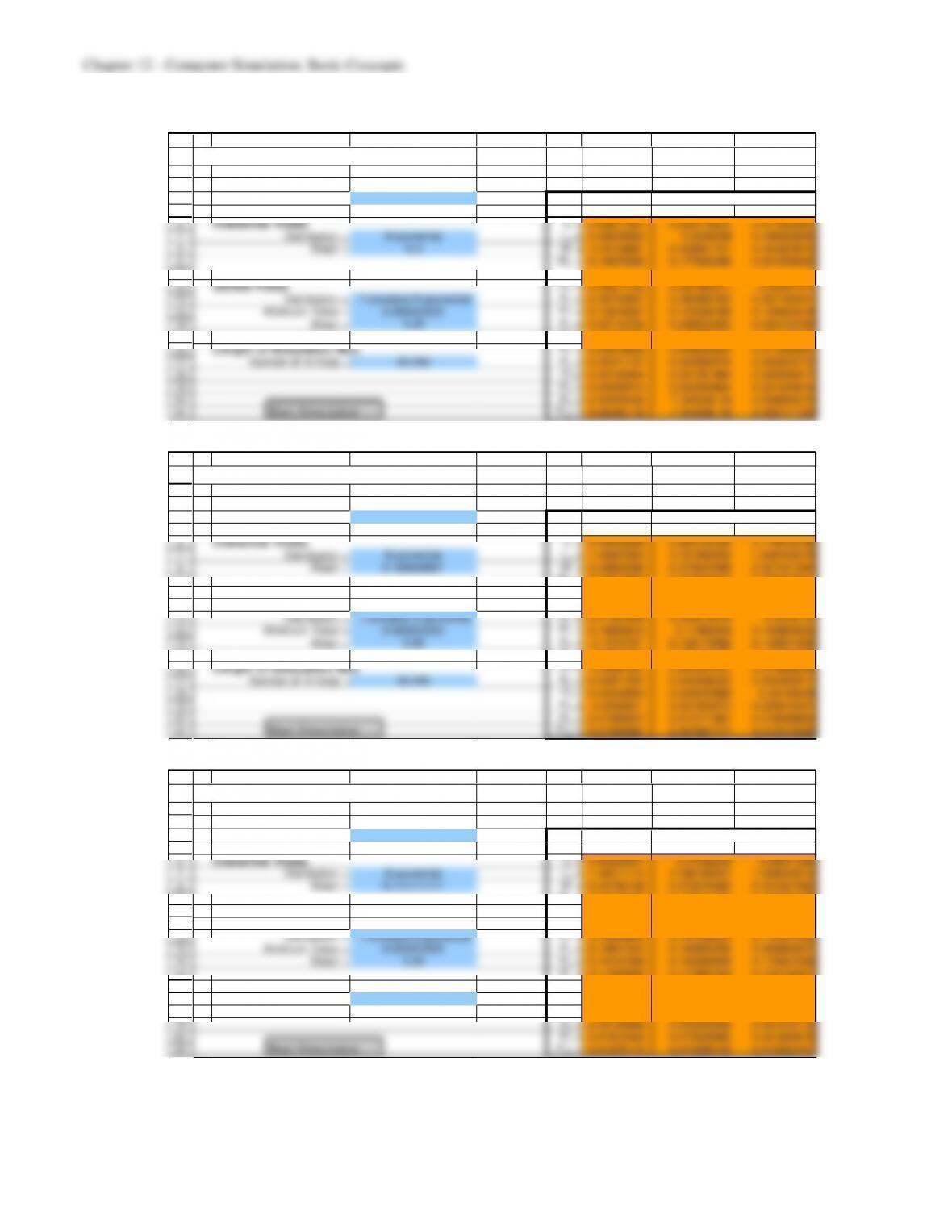
12.20 a) Wq = 0.53 for the simulation run is smaller than for the queueing model (0.75).
1
2
3
4
5
6
7
8
9
10
11
12
13
14
15
16
17
18
19
20
21
A B C D E F G H
Template for Queueing Simulation
Data Results
Number of Servers = 1 Point
Estimate Low High
Interarrival Times L = 2.3056696 2.128818557 2.482520634
Distribution = Exponential Lq = 1.56263017 1.393635616 1.731624718
Mean = 0.333333333 W = 0.77566478 0.721711828 0.829617727
0.9 Wq = 0.52569422 0.472536326 0.578852114
Service T imes P0 = 0.25696057 0.246016915 0.267904228
Distribution = Translated Exponential P1 = 0.23790698 0.229376715 0.246437242
Minimum Value = 0.083333333 P2 = 0.16640728 0.160785864 0.172028692
Mean = 0.25 P3 = 0.11160929 0.106795402 0.116423176
P4 = 0.07359647 0.068895529 0.07829742
Length of Simu lation Run P5 = 0.04884347 0.044496436 0.053190508
Number of Arrivals = 25,000 P6 = 0.03498426 0.031150805 0.038817711
P7
=0.02254759 0.019325189 0.025769993
P8 = 0.01482942 0.012189754 0.017469087
P9 = 0.0096031 0.007252467 0.011953737
P10 = 0.00612262 0.004291876 0.007953356
95% Confidence Interval
Run Simulation
12–26
b) Wq = 0.19 for the simulation run is smaller than for the queueing model (0.25).
1
2
3
4
5
6
7
8
9
10
11
12
13
14
15
16
17
18
19
20
21
A B C D E F G H
Template for Queueing Simulation
Data Results
Number of Servers = 1 Point
Estimate Low High
Interarrival Times L = 0.88511961 0.852718633 0.917520587
Distribution = Exponential Lq = 0.38029663 0.3540296 0.406563666
Mean = 0.5 W = 0.4415882 0.428651721 0.454524674
0.9 Wq = 0.18973086 0.177922488 0.201539232
Service T imes P0 = 0.49517702 0.487380277 0.50297377
Distribution = Translated Exponential P1 = 0.28703957 0.282884705 0.291194441
Minimum Value = 0.083333333 P2 = 0.12674567 0.123090766 0.130400574
Mean = 0.25 P3 = 0.05116784 0.048202493 0.054133189
P4 = 0.02198329 0.01981653 0.024150041
Length of Simu lation Run P5 = 0.00974806 0.008209524 0.011286587
Number of Arrivals = 25,000 P6 = 0.00471187 0.003582976 0.005840772
P7
=0.00193064 0.001261965 0.002599317
P8 = 0.00092514 0.000449664 0.001400616
P9 = 0.00048406 7.35502E-05 0.000894575
P10 = 8.6834E-05 1.94469E-06 0.000171723
95% Confidence Interval
Run Simulation
c) Wq = 0.25 for the simulation run is smaller than for the queueing model (0.32).
1
2
3
4
5
6
7
8
9
10
11
12
13
14
15
16
17
18
19
20
21
A B C D E F G H
Template for Queueing Simulation
Data Results
Number of Servers = 2 Point
Estimate Low High
Interarrival Times L = 3.00056898 2.826159169 3.174978798
Distribution = Exponential Lq = 1.48907864 1.331992055 1.646165218
Mean = 0.166666667 W = 0.49604286 0.470644268 0.521441444
0.9 Wq = 0.24616892 0.221840015 0.270497821
Service T imes P0 = 0.13726653 0.129521096 0.145011968
Distribution = Translated Exponential P1 = 0.21397659 0.204579478 0.2233737
Minimum Value = 0.083333333 P2 = 0.18684615 0.17982929 0.193863004
Mean = 0.25 P3 = 0.1374737 0.132115862 0.142831538
P4 = 0.09983294 0.095078489 0.104587399
Length of Simu lation Run P5 = 0.0694165 0.064944761 0.073888249
Number of Arrivals = 25,000 P6 = 0.04971597 0.044936032 0.054495917
P7
=0.03349904 0.029533988 0.03746409
P8 = 0.0252801 0.021543873 0.029016331
P9 = 0.01568537 0.012771881 0.018598864
P10 = 0.01003987 0.007667177 0.012412556
95% Confidence Interval
Run Simulation
d) Wq = 0.15 for the simulation run is smaller than for the queueing model (0.19).
1
2
3
4
5
6
7
8
9
10
11
12
13
14
15
16
17
18
19
20
21
A B C D E F G H
Template for Queueing Simulation
Data Results
Number of Servers = 3 Point
Estimate Low High
Interarrival Times L = 3.60596801 3.31592206 3.89601396
Distribution = Exponential Lq = 1.36211114 1.096180257 1.628042015
Mean = 0.111111111 W = 0.40180198 0.372076482 0.431527482
0.9 Wq = 0.15177588 0.123071254 0.180480499
Service T imes P0 = 0.07546354 0.069904873 0.081022211
Distribution = Translated Exponential P1 = 0.16566853 0.157336034 0.174001023
Minimum Value = 0.083333333 P2 = 0.19841544 0.189865258 0.206965627
Mean = 0.25 P3 = 0.16707398 0.160490928 0.173657028
P4 = 0.11905965 0.113987249 0.124132041
Length of Simu lation Run P5 = 0.08275171 0.077865526 0.087637887
Number of Arrivals = 25,000 P6 = 0.05842463 0.053807906 0.063041346
P7
=0.04016973 0.036016572 0.044322889
P8 = 0.02726968 0.023220236 0.031319116
P9 = 0.01815483 0.015028982 0.021280672
P10 = 0.01275115 0.010082145 0.015420161
95% Confidence Interval
Run Simulation

12–27
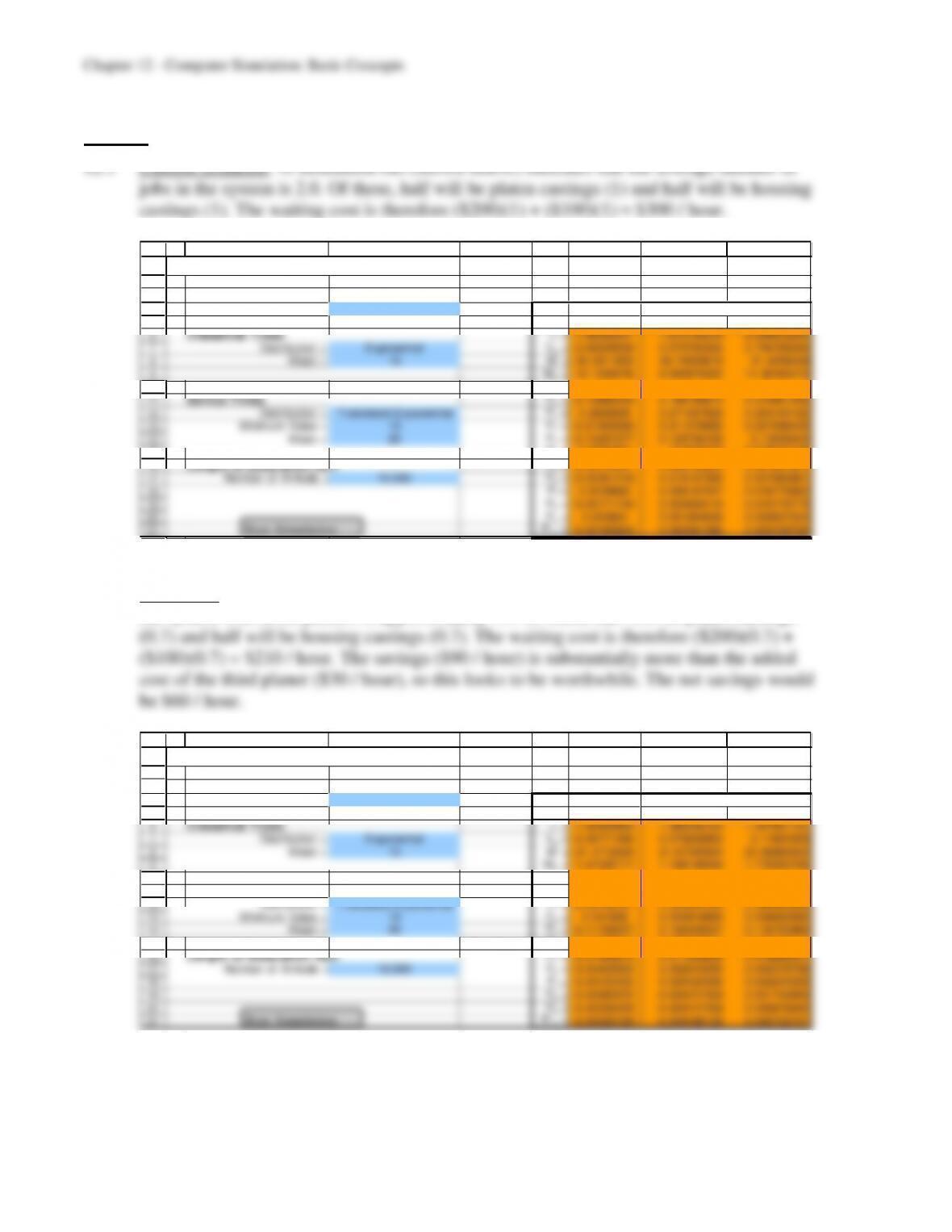
e) The results from a computer simulation can be quite sensitive to the probability
12–28
Cases
1
2
3
4
5
6
7
8
9
10
11
12
13
14
15
16
17
18
19
20
21
A B C D E F G H
Template for Queueing Simulation
Data Results
Number of Servers = 2 Point
Estimate Low High
Interarrival Times L = 1.98365641 1.870700578 2.096612244
Distribution = Exponential Lq = 0.66628639 0.575783306 0.756789465
Mean = 15 W = 30.0811805 28.73655618 31.4258049
5Wq = 10.1039076 8.845870432 11.36194473
Service T imes P0 = 0.19988054 0.188799674 0.210961405
Distribution = T ranslated Exponential P1 = 0.2828689 0.271597628 0.294140162
Minimum Value = 10 P2 = 0.21948306 0.211376682 0.227589435
Mean = 20 P3 = 0.13257277 0.125756108 0.13938943
P4 = 0.0722497 0.0660523 0.078447105
Length o f Simulation Run P5 = 0.04178641 0.036150923 0.047421901
Number of Arrivals = 10,000 P6 = 0.02261418 0.018147395 0.027080961
P7
=0.0129863 0.009197547 0.016775062
P8 = 0.00771744 0.004659116 0.010775773
P9 = 0.003861 0.001884639 0.005837354
P10 = 0.00185903 0.000591296 0.003126755
95% Confidence Interval
Run Simulation
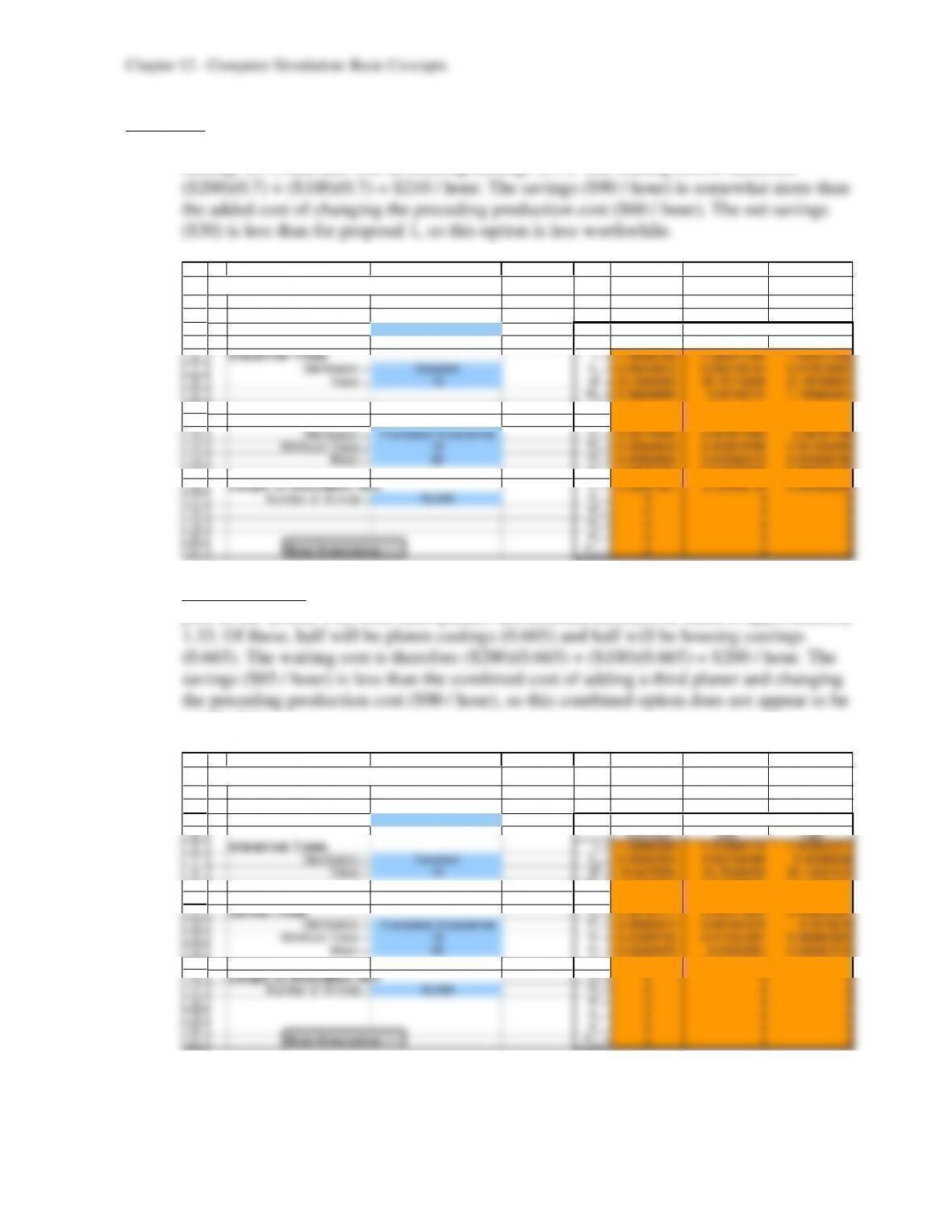
Proposal 1: A simulation run (shown below) indicates that the average number of jobs in
the system with three planers is approximately 1.4. Of these, half will be platen castings
1
2
3
4
5
6
7
8
9
10
11
12
13
14
15
16
17
18
19
20
21
A B C D E F G H
Template for Queueing Simulation
Data Results
Number of Servers = 3 Point
Estimate Low High
Interarrival Times L = 1.42409865 1.380256124 1.467941167
Distribution = Exponential Lq = 0.09771456 0.076609893 0.11881923
Mean = 15 W = 21.4712624 21.07385924 21.86866564
5Wq = 1.47325117 1.168148546 1.778353785
Service T imes P0 = 0.25534157 0.245577077 0.265106061
Distribution = T ranslated Exponential P1 = 0.33796761 0.329893149 0.346042064
Minimum Value = 10 P2 = 0.231656 0.224819899 0.238492092
Mean = 20 P3 = 0.11158027 0.106409547 0.116750986
P4 = 0.04233244 0.038546771 0.046118111
Length o f Simulation Run P5 = 0.01406273 0.011836939 0.016288531
Number of Arrivals = 10,000 P6 = 0.00409905 0.002819395 0.005378708
P7
=0.00133435 0.000425396 0.002243309
P8 = 0.00080672 -0.000131529 0.001744969
P9 = 0.00036429 -0.000147459 0.000876045
P10 = 0.00025729 -0.000188128 0.000702701
95% Confidence Interval
Run Simulation
12–29
Proposal 2: A simulation run (shown below) indicates that the average number of jobs in the
system with constant interarrival times is approximately 1.4. Of these, half will be platen
castings (0.7) and half will be housing castings (0.7). The waiting cost is therefore
1
2
3
4
5
6
7
8
9
10
11
12
13
14
15
16
17
18
19
20
21
A B C D E F G H
Template for Queueing Simulation
Data Results
Number of Servers = 2 Point
Estimate Low High
Interarrival Times L = 1.40396168 1.383412164 1.424511205
Distribution = Constant Lq = 0.06455913 0.055139154 0.073979097
Value = 15 W = 21.0594253 20.75118246 21.36766807
5Wq = 0.96838689 0.82708731 1.109686461
Service T imes P0 = 0.05142644 0.049243293 0.053609594
Distribution = T ranslated Exponential P1 = 0.55774455 0.547877528 0.56761158
Minimum Value = 10 P2 = 0.33345643 0.325678768 0.341234095
Mean = 20 P3 = 0.05060063 0.045262513 0.055938746
P4 = 0.00635733 0.004037203 0.008677449
Length o f Simulation Run P5 = 0.00041461 2.30036E-06 0.000826928
Number of Arrivals = 10,000 P6 = 0 0 0
P7
=0 0 0
P8 = 0 0 0
P9 = 0 0 0
P10 = 0 0 0
95% Confidence Interval
Run Simulation
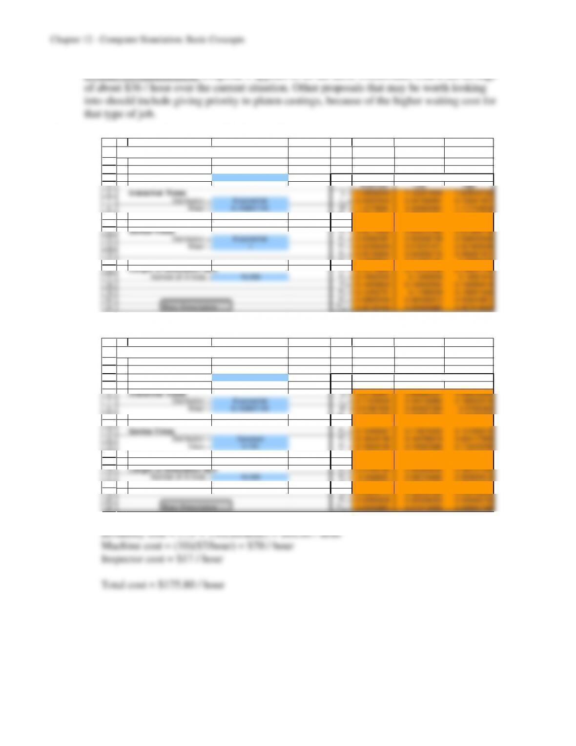
Proposal 1 and 2: A simulation run (shown below) indicates that the average number of
jobs in the system with both three planers and constant interarrival times is approximately
worthwhile.
1
2
3
4
5
6
7
8
9
10
11
12
13
14
15
16
17
18
19
20
21
A B C D E F G H
Template for Queueing Simulation
Data Results
Number of Servers = 3 Point
Estimate Low High
Interarrival Times L = 1.32985569 1.316690172 1.343021211
Distribution = Constant Lq = 0.00052554 0.000184596 0.00086648
Value = 15 W = 19.9478354 19.75035259 20.14531816
5Wq = 0.00788307 0.002768944 0.012997201
Service T imes P0 = 0.05754771 0.055474824 0.059620587
Distribution = T ranslated Exponential P1 = 0.58946474 0.581401676 0.5975278
Minimum Value = 10 P2 = 0.31909725 0.311531281 0.326663225
Mean = 20 P3 = 0.03336476 0.03022801 0.036501519
P4 = 0.00052554 0.000184596 0.00086648
Length o f Simulation Run P5 = 0 0 0
Number of Arrivals = 10,000 P6 = 0 0 0
P7
=0 0 0
P8 = 0 0 0
P9 = 0 0 0
P10 = 0 0 0
95% Confidence Interval
Run Simulation
12–30
Overall recommendation: Proposal 1 appears to be the most worthwhile, with a net savings
12.2 a) Status quo at the presses – 7.5 sheets of in-process inventory.
1
2
3
4
5
6
7
8
9
10
11
12
13
14
15
16
17
18
19
20
21
A B C D E F G H
Template for Queueing Simulation
Data Results
Number of Servers = 10 Point
Estimate Low High
Interarrival Times L = 7.48596004 7.122474949 7.849445126
Distribution = Exponential Lq = 0.55020043 0.347368991 0.753031867
Mean = 0.142857143 W = 1.0770836 1.036422591 1.117744603
5Wq = 0.07916311 0.050901621 0.107424593
Service T imes P0 = 0.00110924 0.000312762 0.001905718
Distribution = Exponential P1 = 0.00582387 0.003292739 0.008355008
Mean = 1 P2 = 0.02306409 0.018701971 0.027426208
25 P3 = 0.05166684 0.043052172 0.060281501
P4 = 0.0866959 0.077527167 0.09586463
Length of Simu lation Run P5 = 0.12118604 0.112124348 0.130247735
Number of Arrivals = 10,000 P6 = 0.14062225 0.13442836 0.14681614
P7
=0.14294653 0.134902634 0.150990419
P8 = 0.12452751 0.11900339 0.130051626
P9 = 0.08806336 0.084082813 0.092043901
P10 = 0.06192446 0.055935883 0.067913035
95% Confidence Interval
Run Simulation
Status quo at the inspection station – 3.6 wing sections of in-process inventory.
1
2
3
4
5
6
7
8
9
10
11
12
13
14
15
16
17
18
19
20
21
A B C D E F G H
Template for Queueing Simulation
Data Results
Number of Servers = 1 Point
Estimate Low High
Interarrival Times L = 3.57765981 3.096884037 4.058435589
Distribution = Exponential Lq = 2.71234549 2.244158962 3.180532014
Mean = 0.142857143 W = 0.51681506 0.454627294 0.57900283
5Wq = 0.39181506 0.329627294 0.45400283
Service T imes P0 = 0.13468567 0.118076335 0.151295015
Distribution = Constant P1 = 0.18444199 0.164766618 0.204117359
Value = 0.125 P2 = 0.16054199 0.145653686 0.175430299
25 P3 = 0.12577666 0.114607169 0.136946159
P4 = 0.09279878 0.083029162 0.102568391
Length of Simu lation Run P5 = 0.07546784 0.065828646 0.085107034
Number of Arrivals = 10,000 P6 = 0.0548405 0.045754492 0.063926513
P7
=0.04326737 0.033313657 0.053221074
P8 = 0.03643173 0.026094365 0.046769093
P9 = 0.02983638 0.020206033 0.039466733
P10 = 0.02245891 0.014710033 0.030207788
95% Confidence Interval
Run Simulation
12–31
b) Proposal 1 will increase the in-process inventory at the presses to 10.6 sheets since the
mean service rate has decreased.
1
2
3
4
5
6
7
8
9
10
11
12
13
14
15
16
17
18
19
20
21
A B C D E F G H
Template for Queueing Simulation
Data Results
Number of Servers = 10 Point
Estimate Low High
Interarrival Times L = 10.6124208 10.07045277 11.15438883
Distribution = Exponential Lq = 2.34034351 1.812410733 2.868276277
Mean = 0.142857143 W = 1.5192496 1.422904809 1.615594383
5Wq = 0.33503816 0.255248897 0.41482742
Service T imes P0 = 0.00034416 -0.000135983 0.000824295
Distribution = Exponential P1 = 0.00330079 0.002146705 0.004454878
Mean = 1.2 P2 = 0.00683624 0.005191338 0.008481139
25 P3 = 0.0225304 0.017788623 0.027272181
P4 = 0.0437143 0.041059108 0.0463695
Length of Simu lation Run P5 = 0.06530488 0.058747044 0.071862716
Number of Arrivals = 10,000 P6 = 0.08305601 0.074729232 0.091382794
P7
=0.09066307 0.081970997 0.099355138
P8 = 0.09495054 0.09393376 0.095967318
P9 = 0.09944674 0.090813615 0.108079863
P10 = 0.08672109 0.077951648 0.095490525
95% Confidence Interval
Run Simulation
The in-process inventory at the inspection station will not change.
This total cost is higher than for the status quo so should not be adopted. The main
reason for the higher cost is that slowing down the machines won’t change in-process
inventory for the inspection station.
12–32
c) Proposal 2 will increase the in-process inventory at the inspection station to 4.2 wing
sections since the variability of the service rate has increased.
1
2
3
4
5
6
7
8
9
10
11
12
13
14
15
16
17
18
19
20
21
A B C D E F G H
Template for Queueing Simulation
Data Results
Number of Servers = 1 Point
Estimate Low High
Interarrival Times L = 4.15349196 3.51945922 4.787524705
Distribution = Exponential Lq = 3.31066782 2.691612222 3.929723426
Mean = 0.142857143 W = 0.58953022 0.506614288 0.672446148
5Wq = 0.46990309 0.387653637 0.552152552
Service T imes P0 = 0.15717586 0.13797724 0.176374483
Distribution = Erlang P1 = 0.16164362 0.143938659 0.179348578
Mean = 0.12 P2 = 0.1417251 0.127306603 0.156143599
k = 2 P3 = 0.11157869 0.100074725 0.123082653
P4 = 0.08340382 0.074497166 0.092310469
Length of Simu lation Run P5 = 0.0729656 0.064546969 0.081384232
Number of Arrivals = 10,000 P6 = 0.05422094 0.04655526 0.061886616
P7
=0.04033746 0.033104015 0.047570898
P8 = 0.03068653 0.023437928 0.037935133
P9 = 0.02468793 0.018553583 0.030822285
P10 = 0.02288346 0.016278465 0.029488445
95% Confidence Interval
Run Simulation
The in-process inventory at the presses will not change.
Inventory cost = (7.5 + 4.2)($8/hour) = $93.60 / hour
This total cost is higher than for the status quo so should not be adopted. The main
reason for the higher cost is the increase in the service rate variability (Erlang rather
than constant) and the resulting increase in the in-process inventory.
12–33
1
2
3
4
5
6
7
8
9
10
11
12
13
14
15
16
17
18
19
20
21
A B C D E F G H
Template for Queueing Simulation
Data Results
Number of Servers = 10 Point
Estimate Low High
Interarrival Times L = 5.74237458 5.581608211 5.903140941
Distribution = Exponential Lq = 0.11624317 0.076181593 0.156304743
Mean = 0.142857143 W = 0.81487258 0.801697429 0.828047729
5Wq = 0.01649551 0.011001805 0.021989206
Service T imes P0 = 0.00445475 0.002433487 0.00647602
Distribution = Exponential P1 = 0.0241519 0.019051394 0.0292524
Mean = 0.8 P2 = 0.06075455 0.0522877 0.069221409
2P3 = 0.10828334 0.096234 0.120332681
P4 = 0.14577459 0.138731319 0.152817867
Length of Simu lation Run P5 = 0.1580859 0.148929657 0.167242144
Number of Arrivals = 10,000 P6 = 0.14882682 0.137378613 0.160275035
P7
=0.12347465 0.116102784 0.13084652
P8 = 0.0909915 0.084900257 0.097082738
P9 = 0.05514285 0.050413495 0.059872212
P10 = 0.03360049 0.029185971 0.038015016
95% Confidence Interval
Run Simulation
This total cost is lower than the status quo and both proposals.