12-1
Chapter 12 Computer Simulation: Basic Concepts
Review Questions
12.1-1 Computer simulation imitates the operation of a stochastic system by using the
corresponding probability distributions to randomly generate the various events that occur
in the system.
12.1-2 Computer simulation typically takes a lot of time and effort, which tends to be relatively
expensive.
12.1-4 A random number is a number between 0 and 1 which is generated in such a way that every
possible number within this interval has an equal chance of occurring. These numbers are
then used to generate random occurrences from probability distributions.
12.2-1 Herr Cutter must decide whether or not to hire an associate.
12.2-3 The probability distributions for service times and interarrival times need to be estimated.
12.2-4 A simulation clock is a variable in the computer program that records how much simulated
time has elapsed.
12.2-6 The state of the system is N(t)=number of customers in the system at time t.
12.3-1 Fritz began by simulating the current operation of the shop. This was largely to test the
validity of his simulation model.
12-2
12.3-4 Fritz’s simulation model assumes that the system has an infinite queue and that once
started, the system operates continually without ever closing and reopening. A simulation
12.4-1 The management science team needs to begin by meeting with management.
12.4-3 A general-purpose simulation language is capable of programming almost any kind of
simulation model. Applications-oriented simulators are designed for simulating fairly
specific types of systems.
12.4-5 Will the measures of performance for the real system be closely approximated by the
values of these measures generated by the simulation model?
12.4-7 The output from the simulation run now provide statistical estimates of the desired
measures of performance for each system configuration of interest.
Problems
12.1 a) Let the numbers 0.0000 to 0.4999 correspond to heads and the numbers 0.5000 to
0.9999 correspond to tails. The random observations for throwing an unbiased coin are
c) Let the numbers 0.0000 to 0.3999 correspond to green lights, the numbers 0.4000 to
0.4999 correspond to yellow lights, and the numbers 0.5000 to 0.9999 correspond to
12.2 a) Answers will vary.
12-3
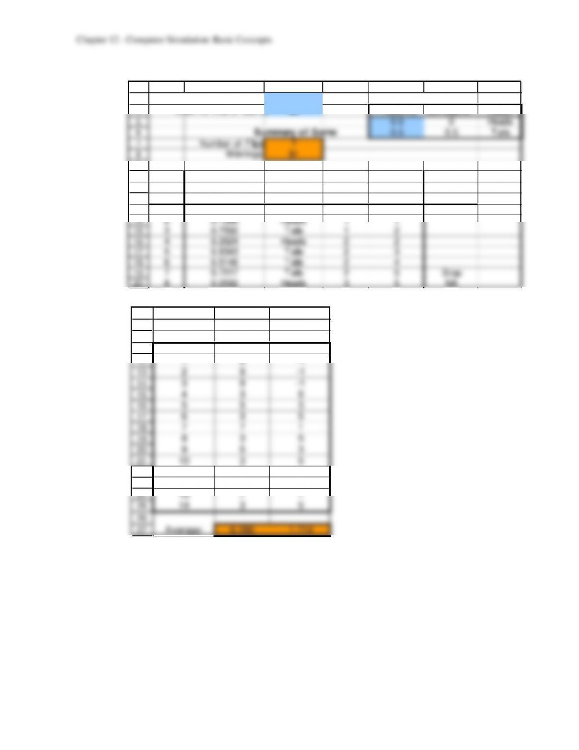
b) The formula in cell D13 is =VLOOKUP(C13, $G$5:$H$6, 2).
3
4
5
6
7
8
9
10
11
12
13
14
15
16
17
18
19
20
B C D E F G H
Required Difference 3 Distribution of Coin Flips
Cash At End of Game $8 Probability Cumulative Result
0.5 0 Heads
Summary of Game 0.5 0.5 Tails
Number of Flips 7
Winnings $1
Random Total Total
Flip Number Result Heads Tails Stop?
1 0.5440 Tails 0 1
2 0.1288 Heads 1 1
3 0.7592 Tails 1 2
4 0.2624 Heads 2 2
5 0.8343 Tails 2 3
6 0.5146 Tails 2 4
7 0.7217 Tails 2 5 Stop
8 0.2592 Heads 3 5 NA
c) A simulation with 14 replications:
9
10
11
12
13
14
15
16
17
18
19
20
21
22
23
24
25
26
27
I J K
Number
Play of Flips W innings
7 1
1 9 -1
2 9 -1
3 9 -1
4 3 5
5 5 3
6 3 5
7 7 1
8 3 5
9 5 3
10 3 5
11 7 1
12 15 -7
13 7 1
14 3 5
Average: 6.286 1.714
12-4
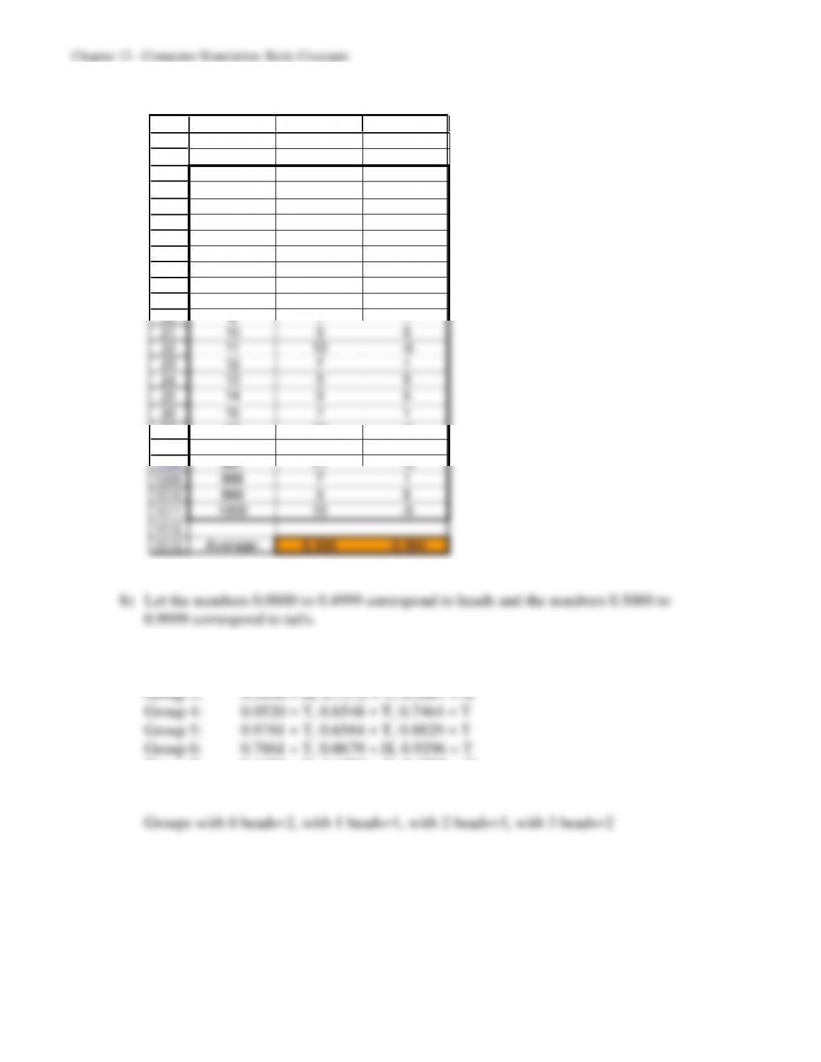
d) A simulation with 1000 replications:
9
10
11
12
13
14
15
16
17
18
19
20
21
22
23
24
25
26
27
28
1008
1009
1010
1011
1012
1013
M N O
Number
Play of Flips W innings
7 1
111 -3
2 3 5
313 -5
4 3 5
527 –19
6 9 -1
7 3 5
811 -3
9 7 1
10 3 5
11 13 -5
12 7 1
13 3 5
14 3 5
15 7 1
16 13 -5
17 5 3
997 11 -3
998 7 1
999 3 5
1000 13 -5
Average: 8.994 –0.994
12.3 a) Answers will vary.
Group 1: 0.7142 = T, 0.4546 = H, 0.3142 = H
Group 2: 0.1722 = H, 0.0932 = H, 0.3645 = H
Group 7: 0.4430 = H, 0.1223 = H, 0.4530 = H
Group 8: 0.3972 = H, 0.9289 = T, 0.2195 = H
12-5
c)
1
2
3
4
5
6
7
A B C
Random
Flip Number Result
1 0.7645 Tails
2 0.8981 Tails
3 0.6682 Tails
Total Number of Heads = 0
d) Answers will vary. The following 8 replications have 0 replications with 0 heads (0/8),
e) Answers will vary. With the following 800 replications, 97 have 0 heads (97/800), 324
have 1 head (324/800), 289 have 2 heads (289/800), and 90 have 3 heads (90/800). This
is quite close to the expected probability distribution.
1
2
3
4
5
6
7
8
9
10
11
12
13
801
802
806
808
H I
Number of
Replication Heads
1
1 1
2 1
3 0
4 2
5 3
6 3
7 2
8 3
9 1
10 3
798 1
799 2
12-6
12.4 a) If it is raining then let the numbers 0.0000 to 0.5999 correspond to rain for the next day
Day
Random Number
Weather
1
0.3039
clear
2
0.7914
clear
3
0.8543
rain
4
0.6902
clear
5
0.3004
clear
6
0.0383
clear
7
0.3883
clear
8
0.6052
clear
9
0.2231
clear
10
0.4250
clear
b)
1
2
3
4
5
6
7
8
9
10
11
12
13
14
15
16
17
A B C
If Clear, Prob(Stays Clear) = 0.8
If Rain, Prob(Stays Rain) = 0.6
Random
Day Number W eather
Clear
1 0.4452 Clear
2 0.6563 Clear
3 0.3412 Clear
4 0.8479 Rain
5 0.9757 Clear
6 0.5992 Clear
7 0.7562 Clear
8 0.3957 Clear
9 0.2929 Clear
10 0.9387 Rain
12.5 a)
2
3
4
B C D E
Simulated Toss
Toss Die 1 Die 2 Sum
1 1 3 4
Chapter 12 – Computer Simulation: Basic Concepts
12-7
b) Answers will vary. Here is one simulation of 25 replications.
2
3
4
5
6
7
8
9
10
11
12
13
14
15
16
17
18
19
20
21
22
23
24
25
26
27
28
B C D E
Simulated Tosses
Toss Die 1 Die 2 Sum
1 1 5 6
2 6 1 7
3 2 5 7
4 4 4 8
5 4 3 7
6 1 2 3
7 5 1 6
8 1 6 7
9 2 2 4
10 5 3 8
11 6 4 10
12 4 1 5
13 3 5 8
14 2 5 7
15 2 4 6
16 6 6 12
17 3 2 5
18 5 1 6
19 4 1 5
20 3 4 7
21 1 5 6
22 3 3 6
23 4 4 8
24 1 3 4
25 6 6 12
c) Answers will vary. For these 25 tosses, a loss occurs on toss 2, a win on toss 3, a loss
12.6 a) Prob(2) = 4/25; Prob (3) = 7/25; Prob(4) = 8/25; Prob (5) = 5/25; Prob(6) = 1/25
correspond to 4 stoves, the numbers 0.7600 to 0.9599 correspond to 5 stoves, and the
numbers 0.9600 to 0.9999 correspond to 6 stoves.
12-8
e) Answers will vary. The following 300-day simulation yielded an average demand of
3.617.
1
2
3
4
5
6
7
8
9
299
300
301
302
303
304
A B C D E F G
Random Distribution of
Day Number Demand Demand
1 0.4449 4 Probability Cumulative Demand
2 0.1673 3 0.16 0 2
3 0.9614 6 0.28 0.16 3
4 0.6088 4 0.32 0.44 4
5 0.8904 5 0.20 0.76 5
6 0.1874 3 0.04 0.96 6
7 0.9291 5
297 0.7936 5
298 0.5947 4
299 0.7095 4
300 0.8926 5
Average = 3.617
12.8 The Federal Aviation Administration (FAA) manages air traffic in the national airspace,
including rerouting traffic when adverse weather conditions occur. To improve FAA
operating procedures, a management science team developed a highly complex computer
managers, airlines, and other aircraft operators used to monitor and modify the behavior of
flights under their control.” The FAA then designated a team of aviation experts to evaluate
how well a number of proposed operating procedures performed when running the
important benefit to passengers.
Computer simulation is continuing to be applied in this way to analyze additional FAA
12.9 a) 3 + 5(0.6505) = 6.25
b) Average = 5.88 which is higher that the mean of 5.5
12–10
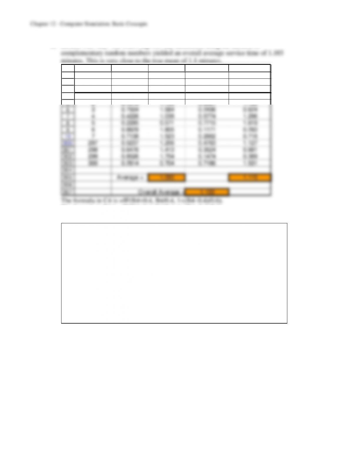
e) Results will vary. The following 300-day simulation using the method of
1
2
3
4
5
6
7
8
9
10
300
301
302
303
304
305
306
307
A B C D E
Complimentary Complimentary
Random Service Random Service
Day Number Time Number Time
1 0.2914 0.729 0.7086 1.514
2 0.4919 1.153 0.5081 1.180
3 0.7504 1.584 0.2496 0.624
4 0.4226 1.038 0.5774 1.296
5 0.2285 0.571 0.7715 1.619
6 0.8829 1.805 0.1171 0.293
7 0.7138 1.523 0.2862 0.716
297 0.5237 1.206 0.4763 1.127
298 0.6476 1.413 0.3524 0.881
299 0.8526 1.754 0.1474 0.369
300 0.2814 0.704 0.7186 1.531
Average = 1.090 1.115
Overall Average = 1.103
The formula in C4 is =IF(B4<0.4, B4/0.4, 1+(B4–0.4)/0.6).
The formula in E4 is =IF(D4<0.4, D4/0.4, 1+(D4–0.4)/0.6).
12.11 a)
12–11
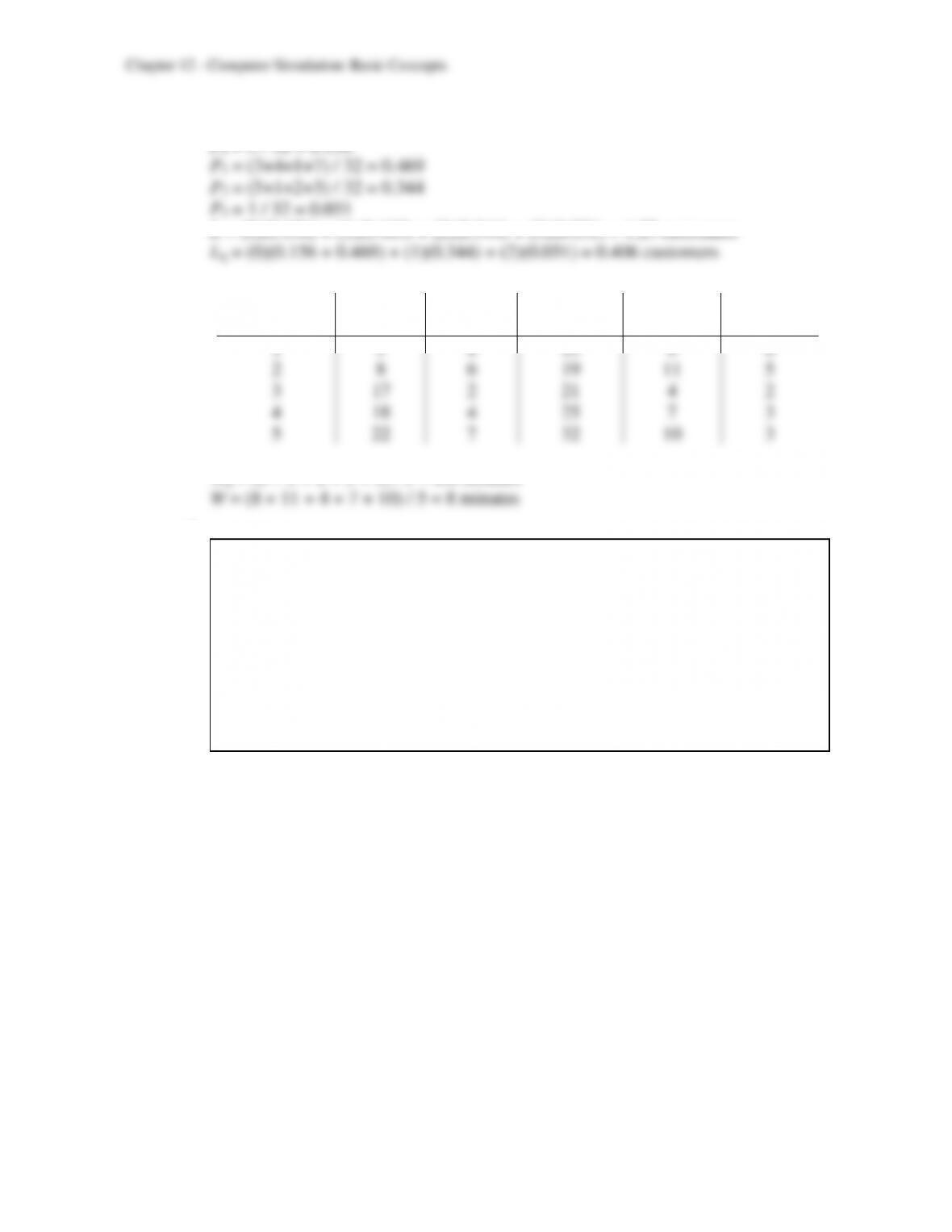
b) Estimates:
P0 = 5 / 32 = 0.156
Customer
Arrival
Time
Service
Time
Departure
Time
System
Time
Wait
Time
1
5
8
13
8
0
2
8
6
19
11
5
3
17
2
21
4
2
4
18
4
25
7
3
5
22
7
32
10
3
Wq = (0 + 5 + 2 + 3 + 3) / 5 = 2.6 minutes
c)
12–12
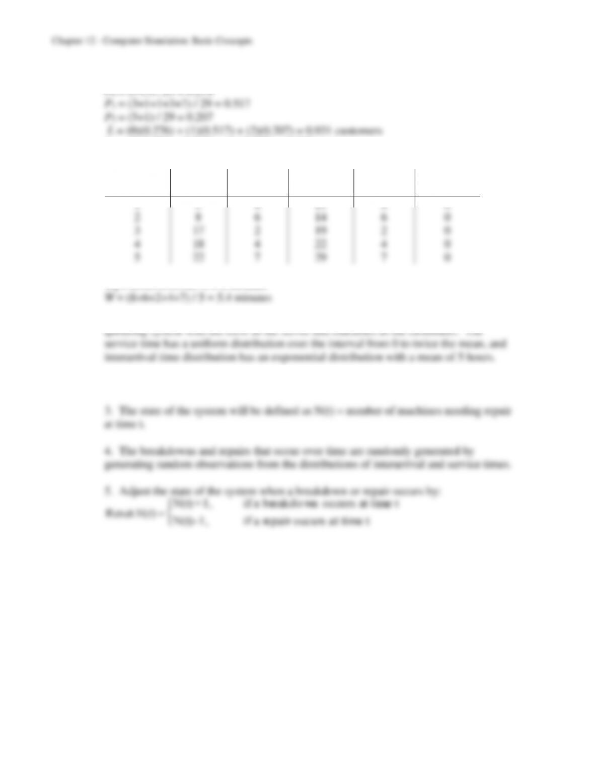
d) Estimates:
Lq = (0)(0.276 + 0.517) + (1)(0.207) = 0.207 customers
Customer
Arrival
Time
Service
Time
Departure
Time
System
Time
Wait
Time
1
5
8
13
8
0
2
8
6
14
6
0
3
17
2
19
2
0
4
18
4
22
4
0
5
22
7
29
7
0
Wq = (0+0+0+0+0) / 5 = 0 minutes
12.12 a) 1. A description of the components of the system. The system is a single-server
2. A simulation clock will record the amount of simulated time that will elapse.
N(t)–1, if a repair occurs at time t
6. Advance the time on the simulation clock by using the next-event time advance
procedure.
12–13
b) 2 Servers:
1
2
3
4
5
6
7
8
9
10
11
12
13
14
15
108
109
110
A B C D E F G H
Mean Interarrival Time = 5 hours
Size of Crew = 2
Mean Service Time = 4 hours
Average Time in Line (W q) = 9.8 hours
Average Time in System (W ) = 13.8 hours
Time Time Time Time Time
Customer Interarrival of Service Service Service in in
Arrival Time Arrival Begins Time Ends Line System
1 0.2 0.2 0.2 0.7 0.8 0.0 0.7
2 5.7 5.9 5.9 5.3 11.2 0.0 5.3
3 5.7 11.6 11.6 0.6 12.2 0.0 0.6
4 12.8 24.4 24.4 2.4 26.8 0.0 2.4
5 19.4 43.8 43.8 7.1 51.0 0.0 7.1
98 6.3 507.0 530.6 0.6 531.1 23.6 24.1
99 1.1 508.1 531.1 2.2 533.3 23.0 25.2
100 1.4 509.5 533.3 7.1 540.4 23.8 30.9
3 Servers:
1
2
3
4
5
6
7
8
9
10
11
12
13
14
15
108
109
110
A B C D E F G H
Mean Interarrival Time = 5 hours
Size of Crew = 3
Mean Service Time = 3 hours
Average Time in Line (W q) = 2.6 hours
Average Time in System (W ) = 5.5 hours
Time T ime Time Time T ime
Customer Interarrival of Service Service Service in in
Arrival Time Arrival Begins Time Ends Line System
1 17.0 17.0 17.0 0.8 17.9 0.0 0.8
2 2.3 19.3 19.3 0.1 19.4 0.0 0.1
3 6.1 25.3 25.3 1.7 27.0 0.0 1.7
4 4.1 29.4 29.4 3.4 32.8 0.0 3.4
5 9.0 38.5 38.5 4.5 42.9 0.0 4.5
98 1.0 482.3 486.4 2.6 489.0 4.0 6.7
99 6.0 488.4 489.0 4.2 493.2 0.6 4.8
100 5.5 493.8 493.8 0.1 494.0 0.0 0.1
4 Servers:
1
2
3
4
5
6
7
8
9
10
11
12
13
14
15
108
109
110
A B C D E F G H
Mean Interarrival Time = 5 hours
Size of Crew = 4
Mean Service Time = 2 hours
Average Time in Line (W q) = 1.9 hours
Average Time in System (W ) = 3.9 hours
Time Time Time Time Time
Customer Interarrival of Service Service Service in in
Arrival Time Arrival Begins Time Ends Line System
1 0.5 0.5 0.5 0.4 0.9 0.0 0.4
2 2.2 2.7 2.7 2.7 5.3 0.0 2.7
3 14.8 17.5 17.5 0.3 17.7 0.0 0.3
4 1.1 18.5 18.5 3.2 21.8 0.0 3.2
5 4.2 22.8 22.8 3.2 26.0 0.0 3.2
98 0.1 419.6 423.2 2.3 425.5 3.7 5.9
99 7.3 426.8 426.8 3.8 430.6 0.0 3.8
100 2.0 428.8 430.6 3.2 433.8 1.7 5.0
For these simulation runs, 3 servers was enough to get the average waiting time before
12–14
c) 2 Servers:
3
4
5
6
7
8
9
10
11
12
13
14
15
16
17
18
19
20
21
B C D E F G H
Data Resu lts
Number of Servers = 1 Point
Estimate Low High
Interarrival T imes L = 2.6400238 2.391023309 2.889024283
Distribution = Exponential Lq = 1.84604969 1.608885509 2.083213873
Mean = 5 W = 13.1728145 12.0696828 14.27594616
5Wq = 9.21115565 8.123435323 10.29887598
Service T imes P0 = 0.2060259 0.189913768 0.222138023
Distribution = Uniform P1 = 0.21033483 0.19666573 0.224003924
Minimum Value = 0 P2 = 0.17681767 0.166556409 0.187078933
Maximum Value = 8 P3 = 0.129046 0.120983504 0.137108487
P4 = 0.09237515 0.0840719 0.10067841
Leng th o f Simulation Run P5 = 0.05972938 0.052306386 0.067152364
Number of Arrivals = 10,000 P6 = 0.04061194 0.033735507 0.047488372
P7 =0.02570094 0.019924133 0.031477739
P8 = 0.01952973 0.014201062 0.024858396
P9 = 0.01383571 0.008578989 0.019092438
P10 = 0.00887497 0.004710957 0.013038973
95% Confidence Interval
Run Simulation
3 Servers:
3
4
5
6
7
8
9
10
11
12
13
14
15
16
17
18
19
20
21
B C D E F G H
Data Resu lts
Number of Servers = 1 Point
Estimate Low High
Interarrival T imes L = 1.17865593 1.111741567 1.245570292
Distribution = Exponential Lq = 0.58142685 0.524764999 0.638088703
Mean = 5 W = 5.91918526 5.65053463 6.18783588
5Wq = 2.9199134 2.666936281 3.172890524
Service T imes P0 = 0.40277092 0.389560579 0.415981265
Distribution = Uniform P1 = 0.28793502 0.280079418 0.295790626
Minimum Value = 0 P2 = 0.16180994 0.155142676 0.168477212
Maximum Value = 6 P3 = 0.07967267 0.073660996 0.08568435
P4 = 0.03651699 0.031748426 0.041285556
Leng th o f Simulation Run P5 = 0.01757122 0.013322806 0.02181963
Number of Arrivals = 10,000 P6 = 0.00761098 0.00515633 0.010065639
P7 =0.00287097 0.001559445 0.0041825
P8 = 0.00155877 0.000478633 0.002638915
P9 = 0.00102093 0.000143421 0.001898433
P10 = 0.00053959 -4.99843E-05 0.001129168
95% Confidence Interval
Run Simulation
4 Servers:
3
4
5
6
7
8
9
10
11
12
13
14
15
16
17
18
19
20
21
B C D E F G H
Data Resu lts
Number of Servers = 1 Point
Estimate Low High
Interarrival T imes L = 0.58179891 0.557903926 0.605693887
Distribution = Exponential Lq = 0.18464567 0.168481455 0.200809875
Mean = 5 W = 2.91732338 2.835376625 2.999270141
5Wq = 0.92587165 0.855487569 0.996255741
Service T imes P0 = 0.60284676 0.593327724 0.612365793
Distribution = Uniform P1 = 0.26540635 0.259908321 0.270904384
Minimum Value = 0 P2 = 0.0936247 0.088999592 0.098249817
Maximum Value = 4 P3 = 0.02737279 0.024387888 0.030357684
P4 = 0.00779303 0.00605179 0.009534275
Leng th o f Simulation Run P5 = 0.00208646 0.00127293 0.002899985
Number of Arrivals = 10,000 P6 = 0.00067048 0.000184955 0.001156013
P7 =0.00019793 -2.48982E-05 0.00042076
P8 = 1.4939E-06 -1.43181E-06 4.41962E-06
P9 = 0 0 0
P10 = 0 0 0
95% Confidence Interval
Run Simulation
For these simulation runs, 3 servers was enough to get the average waiting time before
12–15
d) 2 Servers:
1
2
3
4
5
6
7
8
A B C D E F G
Template for the M/G/1 Queueing Model
Data Results
= 0.2 (mean arrival rate) L = 2.933333333
= 4 (expected service time) Lq = 2.133333333
= 2.30940108 (standard deviation)
s = 1 (# servers) W = 14.66666667
Wq = 10.66666667
3 Servers:
1
2
3
4
5
6
7
8
A B C D E F G
Template for the M/G/1 Queueing Model
Data Results
= 0.2 (mean arrival rate) L = 1.2
= 3 (expected service time) Lq = 0.6
= 1.73205081 (standard deviation)
s = 1 (# servers) W = 6
Wq = 3
4 Servers:
1
2
3
4
5
6
7
8
A B C D E F G
Template for the M/G/1 Queueing Model
Data Results
= 0.2 (mean arrival rate) L = 0.577777778
= 2 (expected service time) Lq = 0.177777778
= 1.15470054 (standard deviation)
s = 1 (# servers) W = 2.888888889
Wq = 0.888888889
3 servers is enough to get the average waiting time before repair down to 3 hours.
12–16
12.13
Customer
Arrival
Interarrival
Time
Time of
Arrival
Time
Service
Begins
Service
Time
Time
Service
Ends
Time in
Line
Time in
System
1
4.0
4.0
4.0
19.6
23.6
0
19.6
2
15.6
19.6
19.6
24.9
44.5
0
24.9
3
1.4
21.0
23.6
15.7
39.3
2.6
18.3
4
36.0
56.9
56.9
20.9
77.8
0
20.9
5
41.4
98.3
98.3
16.0
114.3
0
16.0
6
30.2
128.6
128.6
18.9
147.5
0
18.9
7
10.0
138.6
138.6
20.6
159.2
0
20.6
8
35.8
174.4
174.4
23.4
197.8
0
23.4
9
13.0
187.4
187.4
18.8
206.2
0
18.8
10
12.0
199.4
199.4
19.2
218.6
0
19.2
a) Only the third customer has to wait before beginning a haircut. He waits for 2.6
minutes.
12.14 a)
12–17
b) Estimates:
c) Estimates:
d) Estimates:
W = (sum of observed times) / (number of observed times)
12.15 AT&T uses a discrete event simulation model to simulate inbound call centers. “The call
processing simulator (CAPS) simulates the interactive behavior of the operational variables
in inbound call centers. AT&T uses CAPS to propose optimal staffing, trunking (number of
phone lines), network routing, and premises routing. CAPS can demonstrate cost/benefit
trade-offs and can show the implications of good versus bad service levels. It can also
As a result of this study, “AT&T has increased, protected, and regained more than $1
billion from a business customer base of about 2,000 accounts per year. Much of its
effective market and revenue-share management results from using CAPS to demonstrate
advanced 800 network features. CAPS is vital to the marketability of such new and