Chapter 11 – Queueing Models
11–21
c) The new proposal shows that they will be slightly worse off if they switch to the new
queueing system.
11.23 a) M/M/s model:
3
4
5
6
7
8
9
10
11
12
13
14
15
16
17
18
19
20
21
22
B C D E G H I
Data Results
= 2 (mean arrival rate) L = 2.173913043
= 1 (mean service rate)
Lq = 0.173913043
s = 4 (# servers)
W = 1.086956522
Pr(W > t) = 0.00790187
Wq = 0.086956522
when t = 5
= 0.5
Prob(Wq
> t) = 7.8956E-06
when t = 5 n
Pncumulative
0 0.130434783 0.130434783
1 0.260869565 0.391304348
2 0.260869565 0.652173913
3 0.173913043 0.826086957
4 0.086956522 0.913043478
5 0.043478261 0.956521739
6 0.02173913 0.97826087
7 0.010869565 0.989130435
8 0.005434783 0.994565217
9 0.002717391 0.997282609
All the guidelines are currently being met. The average number in line is 0.17, 99.7%
b) (M/M/s model):
3
4
5
6
7
8
9
10
11
12
13
14
15
16
17
18
19
20
21
22
B C D E G H I
Data Results
= 3 (mean arrival rate) L = 4.528301887
= 1 (mean service rate)
Lq = 1.528301887
s = 4 (# servers)
W = 1.509433962
Pr(W > t) = 0.02390064
Wq = 0.509433962
when t = 5
= 0.75
Prob(Wq
> t) = 0.00343254
when t = 5 n
Pncumulative
0 0.037735849 0.037735849
1 0.113207547 0.150943396
2 0.169811321 0.320754717
3 0.169811321 0.490566038
4 0.127358491 0.617924528
5 0.095518868 0.713443396
6 0.071639151 0.785082547
7 0.053729363 0.83881191
8 0.040297022 0.879108933
9 0.030222767 0.9093317
The first two guidelines will not be satisfied in one year but the third will be. The
c) Five tellers will be needed in a year to meet all of the requirements (M/M/s model):
3
4
5
6
7
8
9
10
11
12
13
14
15
16
17
18
19
20
21
22
B C D E G H I
Data Results
= 3 (mean arrival rate) L = 3.354227405
= 1 (mean service rate)
Lq = 0.354227405
s = 5 (# servers)
W = 1.118075802
Pr(W > t) = 0.0083184
Wq = 0.118075802
when t = 5
= 0.6
Prob(Wq
> t) = 1.0721E-05
when t = 5 n
Pncumulative
0 0.04664723 0.04664723
1 0.139941691 0.186588921
2 0.209912536 0.396501458
3 0.209912536 0.606413994
4 0.157434402 0.763848397
5 0.094460641 0.858309038
11–23
11.24 a) Increasing the utilization factor increases the length and duration of the queue. The
increases are huge when gets very close to 1.
(M/M/s Model):
3
4
5
6
7
8
9
10
11
12
13
14
39
40
41
42
43
44
B C D E G H
Data Results
= 0.5 (mean arrival rate) L = 1
= 1 (mean service rate)
Lq = 0.5
s = 1 (# servers)
W = 2
Pr(W > t) = 0.082085
Wq = 1
when t = 5
= 0.5
Prob(Wq > t) = 0.0410425
when t = 5 n
Pn
0 0.5
1 0.25
L
LqWWqProb(W > 5)
1 0.5 2 1 0.082085
0.5 1 0.5 2 1 0.082085
0.9 9 8.1 10 9 0.6065307
0.99 99 98.01 100 99 0.9512294
b) Increasing the utilization factor increases the length and duration of the queue. The
increases are huge when gets very close to 1.
(M/M/s Model):
3
4
5
6
7
8
9
10
11
12
13
14
39
40
41
42
L
LqWWqProb(W > 5)
43
44
B C D E G H
Data Results
= 0.5 (mean arrival rate) L = 1.3333333
= 0.5 (mean service rate)
Lq = 0.3333333
s = 2 (# servers)
W = 2.6666667
Pr(W > t) = 0.1504892
Wq = 0.6666667
when t = 5
= 0.5
Prob(Wq > t) = 0.0273617
when t = 5 n
Pn
0 0.3333333
1 0.3333333
0.9 9.4736842 7.6736842 10.526316 8.5263158 0.6410337
0.99 99.497487 97.517487 100.50251 98.502513 0.9556861
11.25 (M/M/1 model):
3
4
5
6
7
8
9
10
11
12
13
14
B C D E G H I
Data Results
= 0.16666667 (mean arrival rate) L = 5
= 0.2 (mean service rate)
Lq = 4.166666667
s = 1 (# servers)
W = 30
Pr(W > t) = 0.71653131
Wq = 25
when t = 10
= 0.833333333
Prob(Wq
> t) = 0.83333333
when t = 0 n
Pncumulative
0 0.166666667 0.166666667
1 0.138888889 0.305555556
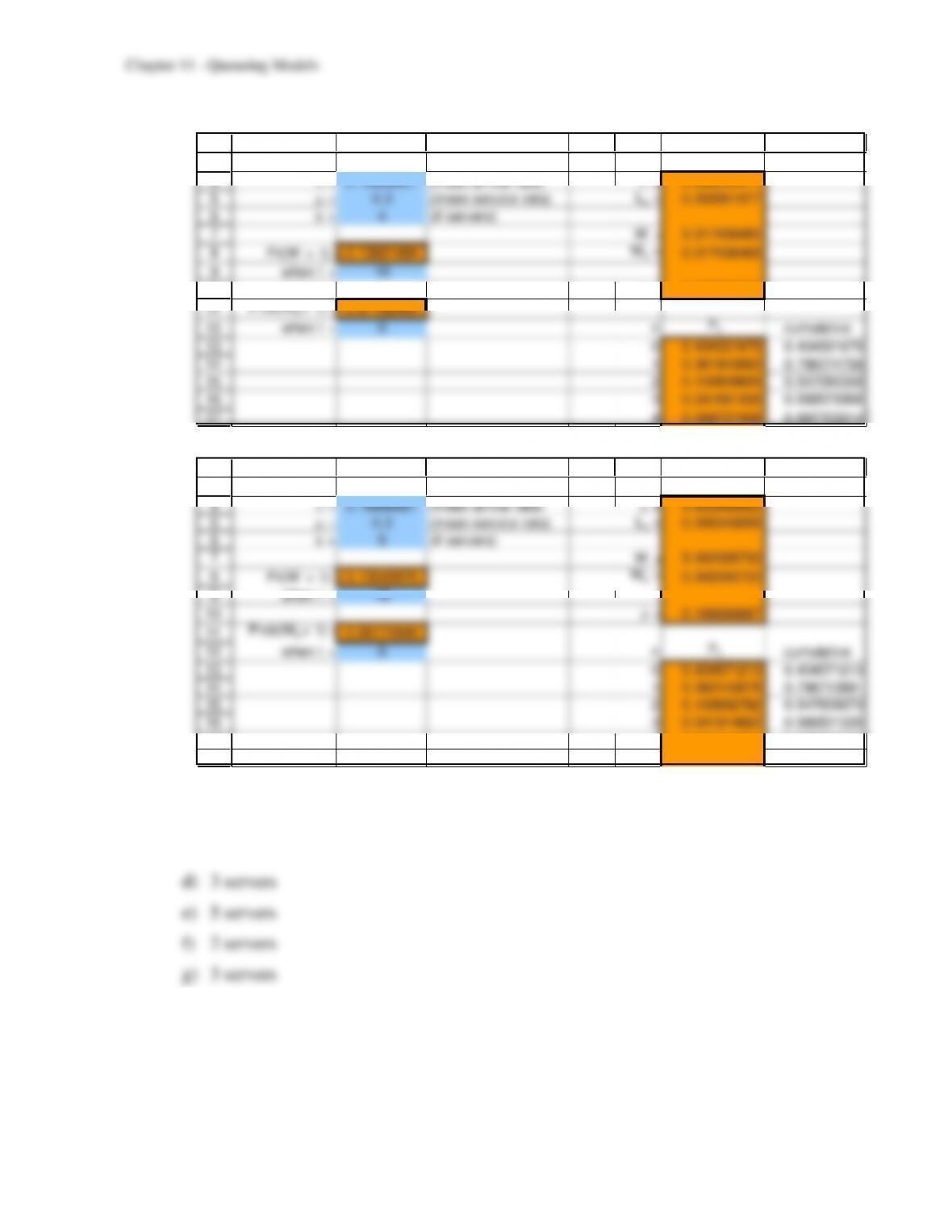
(M/M/2 model):
3
4
5
6
7
8
9
10
11
12
13
14
15
B C D E G H I
Data Results
= 0.16666667 (mean arrival rate) L = 1.008403361
= 0.2 (mean service rate)
Lq = 0.175070028
s = 2 (# servers)
W = 6.050420168
Pr(W > t) = 0.19175192
Wq = 1.050420168
when t = 10
= 0.416666667
Prob(Wq > t) = 0.24509804
when t = 0 n
Pncumulative
0 0.411764706 0.411764706
1 0.343137255 0.754901961
2 0.142973856 0.897875817
(M/M/3 model):
3
4
5
6
7
8
9
10
11
12
13
14
15
16
B C D E G H I
Data Results
= 0.16666667 (mean arrival rate) L = 0.855529512
= 0.2 (mean service rate)
Lq = 0.022196179
s = 3 (# servers)
W = 5.133177072
Pr(W > t) = 0.14138057
Wq = 0.133177072
when t = 10
= 0.277777778
Prob(Wq > t) = 0.05771006
when t = 0 n
Pncumulative
0 0.432132964 0.432132964
1 0.360110803 0.792243767
2 0.150046168 0.942289935
3 0.041679491 0.983969426
(M/M/4 model):
3
4
5
6
7
8
9
10
11
12
13
14
15
16
17
B C D E G H I
Data Results
= 0.16666667 (mean arrival rate) L = 0.836234411
= 0.2 (mean service rate)
Lq = 0.002901077
s = 4 (# servers)
W = 5.017406465
Pr(W > t) = 0.13601484
Wq = 0.017406465
when t = 10
= 0.208333333
Prob(Wq
> t) = 0.01102409
when t = 0 n
Pncumulative
0 0.434331675 0.434331675
1 0.361943063 0.796274738
2 0.150809609 0.947084348
3 0.041891558 0.988975906
4 0.008727408 0.997703314
(M/M/5 model):
3
4
5
6
7
8
9
10
11
12
13
14
15
16
17
18
B C D E G H I
Data Results
= 0.16666667 (mean arrival rate) L = 0.833682622
= 0.2 (mean service rate)
Lq = 0.000349289
s = 5 (# servers)
W = 5.002095733
Pr(W > t) = 0.13540979
Wq = 0.002095733
when t = 10
= 0.166666667
Prob(Wq
> t) = 0.00174644
when t = 0 n
Pncumulative
0 0.434571213 0.434571213
1 0.362142678 0.796713891
2 0.150892782 0.947606673
3 0.041914662 0.989521335
4 0.008732221 0.998253556
5 0.00145537 0.999708926
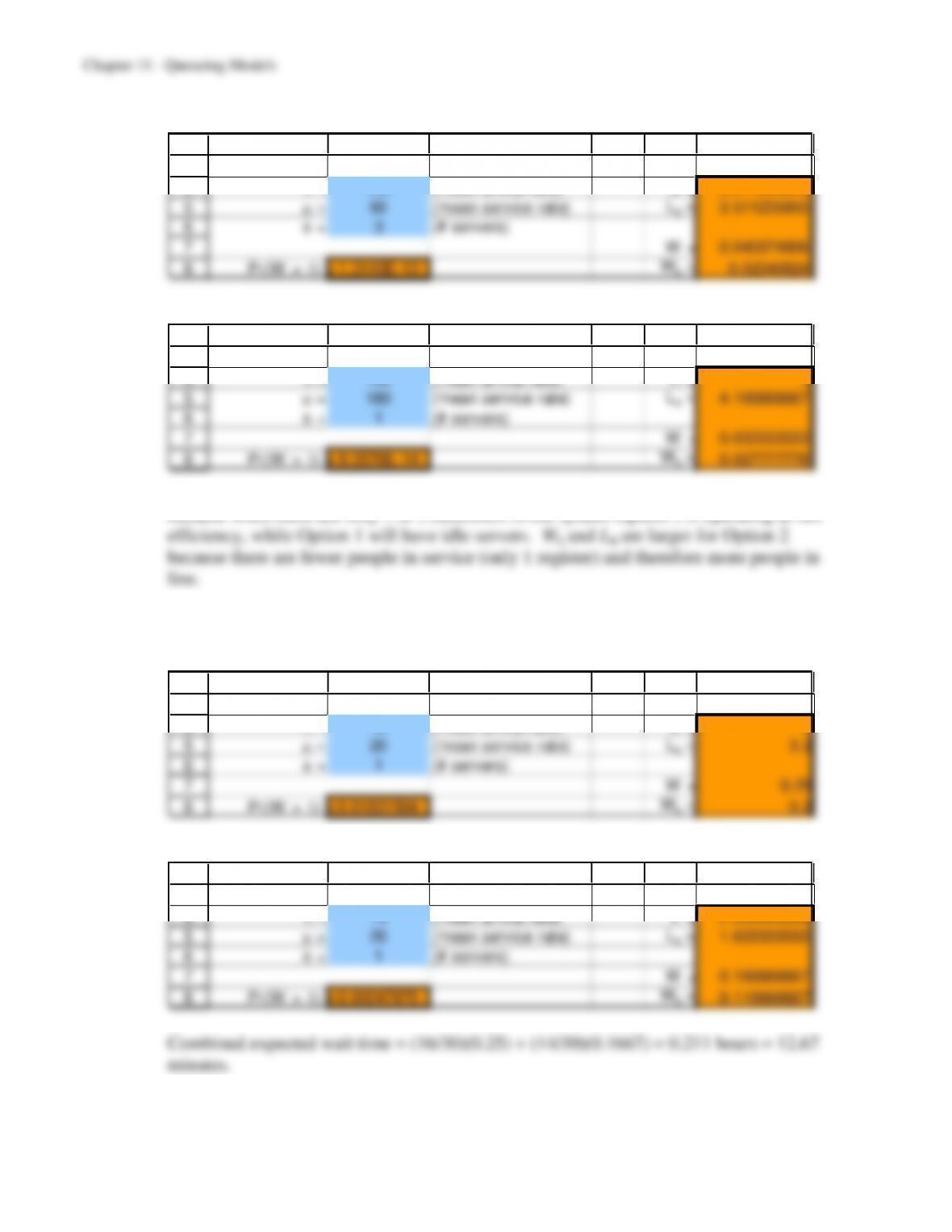
a) 2 servers
b) 3 servers
c) 4 servers
11–26
11.26 a) Option 1 (M/M/3 Model):
3
4
5
6
7
8
B C D E G H
Data Results
= 150 (mean arrival rate) L = 6.011235955
= 60 (mean service rate)
Lq = 3.511235955
s = 3 (# servers)
W = 0.040074906
Pr(W > t) = 1.3143E-13
Wq = 0.02340824
Option 2 (M/M/1 Model):
3
4
5
6
7
8
B C D E G H
Data Results
= 150 (mean arrival rate) L = 5
= 180 (mean service rate)
Lq = 4.166666667
s = 1 (# servers)
W = 0.033333333
Pr(W > t) = 9.3576E-14
Wq = 0.027777778
b) W and L are smaller for Option 2 because it is a more efficient system. This is true
because when there are only 1 or 2 customers in the system Option 2 is operating at full
c) W should be the most important measure to customers since they should be most
concerned with the total time spent in the system. Given this, Option 2 is better.
11.27 a) Deposits:
3
4
5
6
7
8
B C D E G H
Data Results
= 16 (mean arrival rate) L = 4
= 20 (mean service rate)
Lq = 3.2
s = 1 (# servers)
W = 0.25
Pr(W > t) = 0.01831564
Wq = 0.2
Withdrawals:
3
4
5
6
7
8
B C D E G H
Data Results
= 14 (mean arrival rate) L = 2.333333333
= 20 (mean service rate)
Lq = 1.633333333
s = 1 (# servers)
W = 0.166666667
Pr(W > t) = 0.00247875
Wq = 0.116666667
11–27
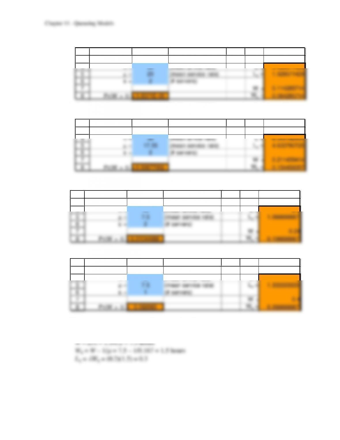
b) Expected waiting time = 0.114 hours = 6.86 minutes.
3
4
5
6
7
8
B C D E G H
Data Results
= 30 (mean arrival rate) L = 3.428571429
= 20 (mean service rate)
Lq = 1.928571429
s = 2 (# servers)
W = 0.114285714
Pr(W > t) = 5.8371E-05
Wq = 0.064285714
c) An expected processing time of 3.42 minutes (17.55 customers per hour) would cause
the expected waiting times to be the same for the two procedures.
3
4
5
6
7
8
B C D E G H
Data Results
= 30 (mean arrival rate) L = 6.343182434
= 17.55 (mean service rate)
Lq = 4.633780725
s = 2 (# servers)
W = 0.211439414
Pr(W > t) = 0.00677002
Wq = 0.154459357
11.28 This year:
3
4
5
6
7
8
B C D E G H
Data Results
= 10 (mean arrival rate) L = 2.4
= 7.5 (mean service rate)
Lq = 1.066666667
s = 2 (# servers)
W = 0.24
Pr(W > t) = 0.01044886
Wq = 0.106666667
Next year:
3
4
5
6
7
8
B C D E G H
Data Results
= 5 (mean arrival rate) L = 2
= 7.5 (mean service rate)
Lq = 1.333333333
s = 1 (# servers)
W = 0.4
Pr(W > t) = 0.082085
Wq = 0.266666667
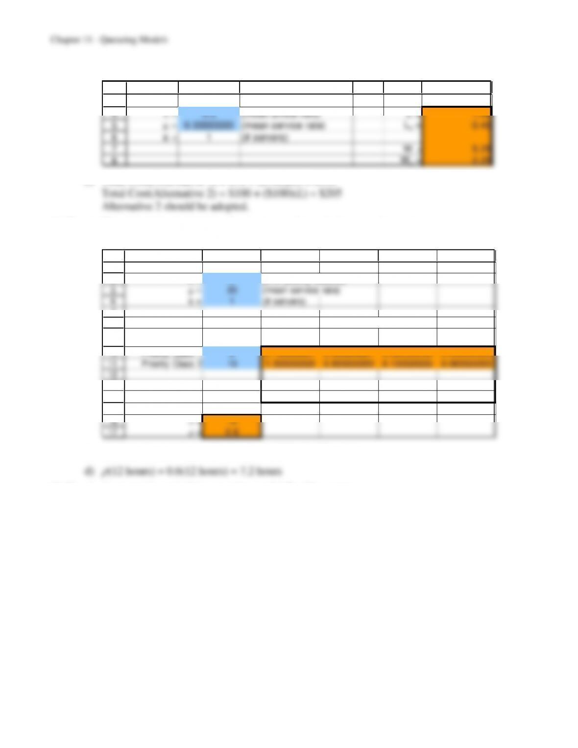
This year’s system yields smaller values for all measure except L.
11.29 a) L = 1.5
b) M/D/1 Model:
3
4
5
6
7
8
B C D E F G
Data Results
= 0.2 (mean arrival rate) L = 1.05
= 0.33333333 (mean service rate)
Lq = 0.45
s = 1 (# servers)
W = 5.25
Wq = 2.25
c) Total Cost(Alternative 1) = $70 + ($100)(L) = $220
11.30 a) This system is an example of a nonpreemptive priority queueing system.
b) M/M/s Nonpreemptive Priority Model:
3
4
5
6
7
8
9
10
11
12
13
14
15
16
17
B C D E F G
Data
n = 2 (# of priority classes)
= 20 (mean service rate)
s = 1 (# servers)
iLLq WWq
Priority Class 1 2 0.166666667 0.066666667 0.083333333 0.033333333
Priority Class 2 10 1.333333333 0.833333333 0.133333333 0.083333333
Priority Class 3 1 0.264285714 0.214285714 0.264285714 0.214285714
Priority Class 4 1 0.335714286 0.285714286 0.335714286 0.285714286
Priority Class 5 1 0.45 0.4 0.45 0.4
= 12
= 0.6
Results
c) Wq(first-class) / Wq(coach-class) = 0.0333 / 0.833 = 0.4
11.31 a) A preemptive priorities queueing model fits this system.
b) M/M/s Preemptive Priority Model:
3
4
5
6
7
8
9
10
11
12
13
14
15
16
B C D E F G
Data
n = 3 (# of priority classes)
= 3 (mean service rate)
s = 1 (# servers)
iLLq WWq
Priority Class 1 0.2 0.071428571 0.004761905 0.357142857 0.023809524
Priority Class 2 0.6 0.292207792 0.092207792 0.487012987 0.153679654
Priority Class 3 1.2 1.636363636 1.236363636 1.363636364 1.03030303
Priority Class 4 1 #DIV/0! #DIV/0! #DIV/0! #DIV/0!
Priority Class 5 1 #DIV/0! #DIV/0! #DIV/0! #DIV/0!
= 2
= 0.666666667
Results
Guidelines will be satisfied next year with a single doctor. The average wait time for
critical cases is 0.024 hours = 1.43 minutes; the average wait time for serious cases is
0.154 hours = 9.22 minutes; the average wait time for stable cases is 1.03 hours.
c) M/M/1 Model:
3
4
5
6
7
8
B C D E G H
Data Results
= 2 (mean arrival rate) L = 2
= 3 (mean service rate)
Lq = 1.333333333
s = 1 (# servers)
W = 1
Pr(W > t) = 0.36787944
Wq = 0.666666667
The guideline for stable cases would be satisfied but the other two would not be.
d)
3
4
5
6
7
8
9
10
11
12
13
14
15
16
B C D E F G
Data
n = 3 (# of priority classes)
= 3 (mean service rate)
s = 1 (# servers)
iLLq WWq
Priority Class 1 0.225 0.081081081 0.006081081 0.36036036 0.027027027
Priority Class 2 0.675 0.347490347 0.122490347 0.514800515 0.181467181
Priority Class 3 1.35 2.571428571 2.121428571 1.904761905 1.571428571
Priority Class 4 1 -16 -16.3333333 –16 –16.3333333
Priority Class 5 1 9.6 9.266666667 9.6 9.266666667
= 2.25
= 0.75
Results
The guidelines are still met. The average wait time for critical cases is 0.027 hours =
11.32 a) M/M/s Nonpreemptive Priority Model (s=4):
3
4
5
6
7
8
9
10
11
12
13
14
15
16
17
B C D E F G
Data
n = 3 (# of priority classes)
= 4 (mean service rate)
s = 4 (# servers)
iLLq WWq
Priority Class 1 6 1.805660377 0.305660377 0.300943396 0.050943396
Priority Class 2 4 1.543396226 0.543396226 0.385849057 0.135849057
Priority Class 3 2 1.179245283 0.679245283 0.589622642 0.339622642
Priority Class 4 1 0.929245283 0.679245283 0.929245283 0.679245283
Priority Class 5 1 1.608490566 1.358490566 1.608490566 1.358490566
= 12
= 0.75
Results
Chapter 11 – Queueing Models
M/M/s Nonpreemptive Priority Model (s=5):
3
4
5
6
7
8
9
10
11
12
13
14
15
16
17
B C D E F G
Data
n = 3 (# of priority classes)
= 4 (mean service rate)
s = 5 (# servers)
iLLq WWq
Priority Class 1 6 1.60120783 0.10120783 0.266867972 0.016867972
Priority Class 2 4 1.134943773 0.134943773 0.283735943 0.033735943
Priority Class 3 2 0.618075802 0.118075802 0.309037901 0.059037901
Priority Class 4 1 0.334339858 0.084339858 0.334339858 0.084339858
Priority Class 5 1 0.362453145 0.112453145 0.362453145 0.112453145
= 12
= 0.6
Results
The guidelines are met with 4 lathes.
5 lathes should be obtained to minimize the expected total cost.
11.33 a) 1 server is optimal.
3
4
5
6
7
8
9
10
11
12
13
14
15
16
18
B C D
Data
= 8 (mean arrival rate)
= 10 (mean service rate)
s = 1 (# servers)
Pr(W > t) = 0.90483742
when t = 0.05
Prob(Wq > t) = 0.72386993
when t = 0.05
Economic Analysis:
Cs = $100.00 (cost / server / unit time)
11–32
b) 2 servers are optimal.
3
4
5
6
7
8
9
10
11
12
13
14
15
16
17
18
19
20
B C D
Data
= 8 (mean arrival rate)
= 10 (mean service rate)
s = 2 (# servers)
Pr(W > t) = 0.67249526
when t = 0.05
Prob(Wq > t) = 0.12544266
when t = 0.05
Economic Analysis:
Cs = $100.00 (cost / server / unit time)
Cw = $100.00 (waiting cost / unit time)
Cost of Service $200.00
Cost of Waiting $95.24
Total Cost $295.24
c) 3 servers are optimal.
3
4
5
6
7
8
9
10
11
12
13
14
15
16
17
18
19
20
B C D
Data
= 8 (mean arrival rate)
= 10 (mean service rate)
s = 3 (# servers)
Pr(W > t) = 0.61839666
when t = 0.05
Prob(Wq > t) = 0.01732012
when t = 0.05
Economic Analysis:
Cs = $10.00 (cost / server / unit time)
Cw = $100.00 (waiting cost / unit time)
Cost of Service $30.00
11.34 Jim should operate 4 cash registers during the lunch hour.
3
4
5
6
7
8
9
10
11
12
13
14
15
16
17
18
19
20
B C D E F G
Data Resu lts
= 66 (mean arrival rate) L = 2.477198599
= 30 (mean service rate)
Lq = 0.277198599
s = 4 (# servers)
W = 0.037533312
Pr(W > t) = 0.26733457
Wq = 0.004199979
when t = 0.05
= 0.55
Prob(Wq > t) = 0.01524213
when t = 0.05 n
Pn
0 0.104562001
Economic Analysis: 1 0.230036403
Cs = $9.00 (cost / server / unit time) 2 0.253040043
Cw = $18.00 (waiting cost / unit time) 3 0.185562698
4 0.102059484
Cost of Service $36.00 5 0.056132716
Cost of W aiting $44.59 6 0.030872994
Total Cost $80.59 7 0.016980147
11.35 Garrett-Tompkins should have 6 copiers.
3
4
5
6
7
8
9
10
11
12
13
14
15
16
17
18
19
20
B C D E F G
Data Resu lts
= 30 (mean arrival rate) L = 2.533889152
= 12 (mean service rate)
Lq = 0.033889152
s = 6 (# servers)
W = 0.084462972
Pr(W > t) = 0.55690297
Wq = 0.001129638
when t = 0.05
= 0.416666667
Prob(Wq > t) = 0.00580992
when t = 0.05 n
Pn
0 0.081620259
Economic Analysis: 1 0.204050648
Cs = $1.50 (cost / server / unit time) 2 0.25506331
Cw = $25.00 (waiting cost / unit time) 3 0.212552759
4 0.132845474
Cost of Service $9.00 5 0.066422737
Cost of W aiting $63.35 6 0.02767614
Total Cost $72.35 7 0.011531725
Cases
11.1 The operations of the records and benefits call center can be modeled as an M/M/s
19
20
21
22
23
a) In order to solve this problem we have to determine the number of servers by “trial and
For 13 servers, the probability that a customer has to wait more than 4 minutes equals
36.3%. It appears that Mark currently employs 13 servers.
1
2
3
4
5
6
7
8
9
10
11
12
13
14
15
16
17
18
19
20
21
22
23
A B C D E G H
Template for the M/M/s Queueing Model
Data Results
= 70 (mean arrival rate) L = 17.07963527
= 6 (mean service rate)
Lq = 5.4129686
s = 13 (# servers)
W = 0.24399479
Pr(W > t) = 0.8256082
Wq = 0.077328123
when t = 0.06666667
= 0.897435897
Prob(Wq > t) = 0.36291401
when t = 0.06666667 n
Pn
0 5.32592E–06
1 6.21358E–05
2 0.000362459
3 0.001409561
4 0.004111221
5 0.009592849
6 0.018652761
7 0.031087935
8 0.045336573
9 0.058769631
10 0.06856457
0
0.01
0.02
0.03
0.04
0.05
0.06
0.07
0.08
0 1 2 3 4 5 6 7 8 9 10 11 12 13 14 15 16 17 18 19 20 21 22 23 24 25
Number of Customers in System
Probability
1
2
3
4
5
6
7
8
9
10
11
12
13
14
15
16
17
18
A B C D E G H
Template for the M/M/s Queueing Model
Data Results
= 70 (mean arrival rate) L = 11.77798802
= 6 (mean service rate)
Lq = 0.111321353
s = 18 (# servers)
W = 0.168256972
Pr(W > t) = 0.90907539
Wq = 0.001590305
when t = 0.01666667
= 0.648148148
Prob(Wq > t) = 0.03207826
when t = 0.01666667 n
Pn
0 8.49029E–06
1 9.90534E–05
2 0.000577812
3 0.002247045
4 0.006553882
5 0.015292391
0.06
0.08
0.1
0.12
0.14
Probability
c) Using the same “trial and error” method as before, we find the minimal number of
1
2
3
4
5
6
7
8
9
10
11
12
13
14
15
16
17
18
19
20
21
22
23
A B C D E G H
Template for the M/M/s Queueing Model
Data Results
= 70 (mean arrival rate) L = 12.61532951
= 6 (mean service rate)
Lq = 0.948662841
s = 15 (# servers)
W = 0.180218993
Pr(W > t) = 0.92671158
Wq = 0.013552326
when t = 0.01666667
= 0.777777778
Prob(Wq > t) = 0.19421332
when t = 0.01666667 n
Pn
0 7.80062E–06
1 9.10072E–05
2 0.000530875
3 0.002064516
4 0.006021504
5 0.014050177
6 0.027319789
7 0.045532982
8 0.066402265
9 0.08607701
10 0.100423178
0
0.02
0.04
0.06
0.08
0.1
0.12
0 1 2 3 4 5 6 7 8 9 10 11 12 13 14 15 16 17 18 19 20 21 22 23 24 25
Number of Customers in System
Probability
The minimal number of servers to ensure that 95% of customers wait 90 seconds or less
is s = 17.
1
2
3
4
5
6
7
8
9
10
11
12
13
14
15
16
17
18
19
20
21
22
23
A B C D E G H
Template for the M/M/s Queueing Model
Data Results
= 70 (mean arrival rate) L = 11.89284685
= 6 (mean service rate)
Lq = 0.226180186
s = 17 (# servers)
W = 0.169897812
Pr(W > t) = 0.8705238
Wq = 0.003231146
when t = 0.025
= 0.68627451
Prob(Wq > t) = 0.04645911
when t = 0.025 n
Pn
0 8.39517E–06
1 9.79436E–05
2 0.000571338
3 0.002221869
4 0.006480452
5 0.015121055
6 0.029402052
7 0.049003419
8 0.07146332
9 0.092637637
10 0.108077243
0
0.02
0.04
0.06
0.08
0.1
0.12
0.14
0 1 2 3 4 5 6 7 8 9 10 11 12 13 14 15 16 17 18 19 20 21 22 23 24 25
Number of Customers in System
Probability
When an employee of Cutting Edge calls the benefits center from work and has to wait
on the phone, the company loses valuable work time for this customer. Mark should try
to estimate the amount of work time employees lose when they have to wait on the
Clearly, Mark’s criteria would be different if he were dealing with external customers.
While the internal customers might become disgruntled when they have to wait on the
phone, they cannot call somewhere else. Effectively, the benefits center holds
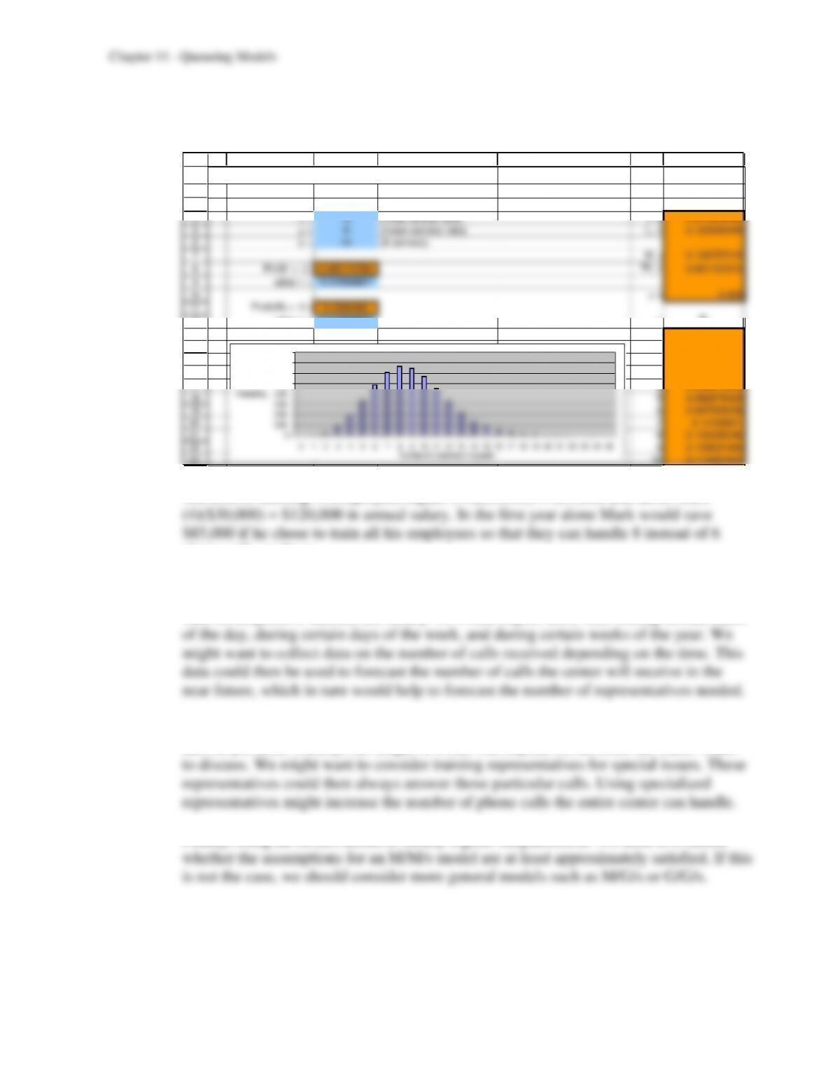
d) If the representatives can only handle 6 calls per hour, then Mark needs to employ 18
representatives (see part b). If a representative can handle 8 calls per hour, then the
minimal number of representatives equals 14.
1
2
3
4
5
6
7
8
9
10
11
12
13
14
15
16
17
18
19
20
21
22
23
A B C D E G H
Template for the M/M/s Queueing Model
Data Results
= 70 (mean arrival rate) L = 8.873005049
= 8 (mean service rate)
Lq = 0.123005049
s = 14 (# servers)
W = 0.126757215
Pr(W > t) = 0.88174766
Wq = 0.001757215
when t = 0.01666667
= 0.625
Prob(Wq > t) = 0.0366495
when t = 0.01666667 n
Pn
0 0.000156459
1 0.001369018
2 0.005989453
3 0.017469238
4 0.038213959
5 0.066874429
6 0.097525208
7 0.12190651
8 0.133335246
9 0.129631489
10 0.113427553
0
0.02
0.04
0.06
0.08
0.1
0.12
0.14
0.16
0 1 2 3 4 5 6 7 8 9 10 11 12 13 14 15 16 17 18 19 20 21 22 23 24 25
Number of Customers in System
Probability
The cost of training 14 employees equals (14)($2,500) = $35,000 and saves Mark
phone calls per hour.
e) Mark needs to carefully check the number of calls arriving at the call center per hour.
In this case we have made the simplifying assumption that the arrival rate is constant.
That assumption is unrealistic; clearly we would expect more calls during certain times
Also, Mark should carefully check the number of phone calls a representative can
answer per hour. Clearly, the length of a call will depend on the issue the caller wants
11–38
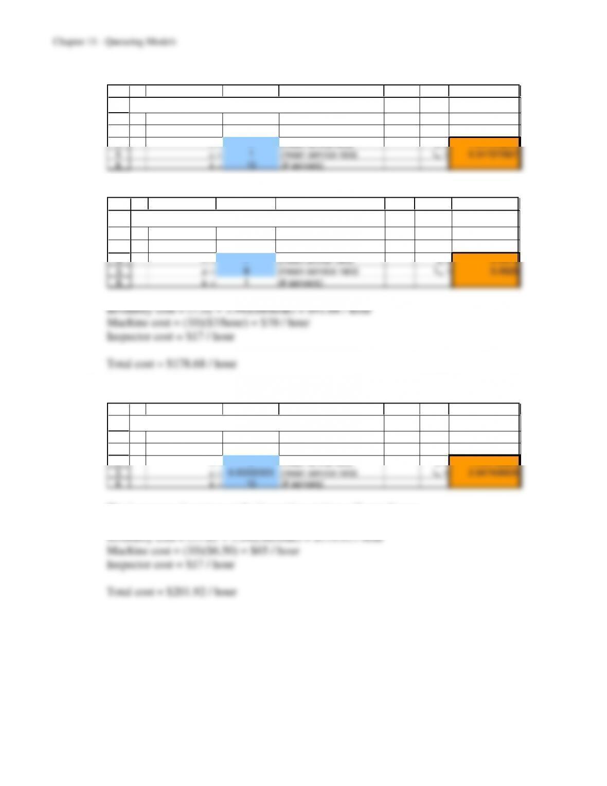
11.2 a) Status quo at the presses – 7.52 sheets of in-process inventory.
1
2
3
4
5
6
A B C D E G H
Template for the M/M/s Queueing Model
Data Results
= 7 (mean arrival rate) L = 7.517372837
= 1 (mean service rate)
Lq = 0.517372837
s = 10 (# servers)
Status quo at the inspection station – 3.94 wing sections of in-process inventory.
1
2
3
4
5
6
A B C D E F G
Template for M/D/1 Queueing Model
Data Results
= 7 (mean arrival rate) L = 3.9375
= 8 (mean service rate)
Lq = 3.0625
s = 1 (# servers)
b) Proposal 1 will increase the in-process inventory at the presses to 11.05 sheets since the
mean service rate has decreased.
1
2
3
4
5
6
A B C D E G H
Template for the M/M/s Queueing Model
Data Results
= 7 (mean arrival rate) L = 11.04740664
= 0.83333333 (mean service rate)
Lq = 2.647406638
s = 10 (# servers)
The in-process inventory at the inspection station will not change.
This total cost is higher than for the status quo so should not be adopted. The main
reason for the higher cost is that slowing down the machines won’t change in-process
inventory for the inspection station.
11–39
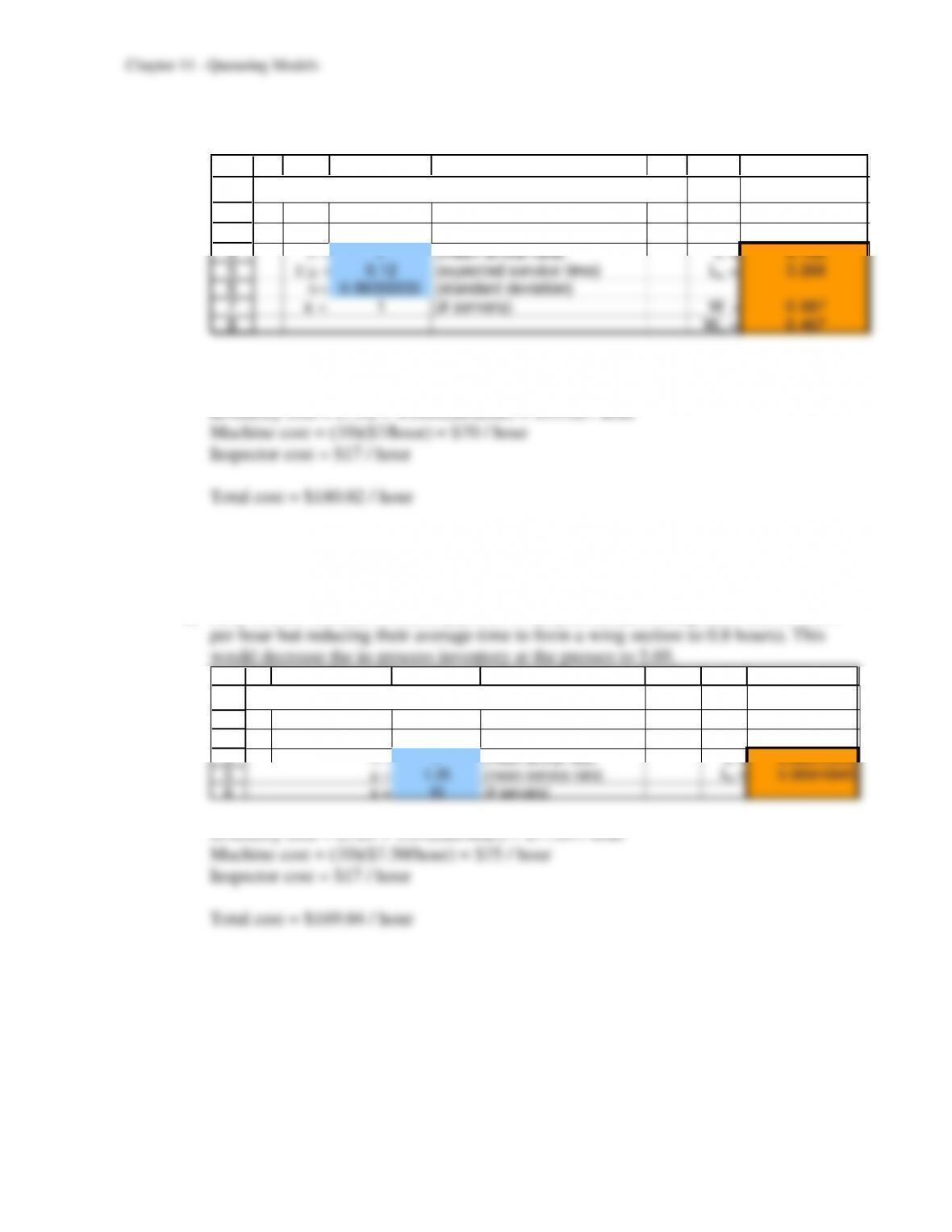
c) Proposal 2 will increase the in-process inventory at the inspection station to 4.108 wing
sections since the variability of the service rate has increased.
1
2
3
4
5
6
7
8
A B C D E F G
Template for the M/G/1 Queueing Model
Data Results
= 7 (mean arrival rate) L = 4.108
= 0.12 (expected service time) Lq = 3.268
= 0.08333333 (standard deviation)
s = 1 (# servers) W = 0.587
Wq = 0.467
The in-process inventory at the presses will not change.
Inventory cost = (7.52 + 4.108)($8/hour) = $93.02 / hour
This total cost is higher than for the status quo so should not be adopted. The main
reason for the higher cost is the increase in the service rate variability and the resulting
increase in the in-process inventory.
d) They should consider increasing power to the presses (increasing there cost to $7.50
1
2
3
4
5
6
A B C D E G H
Template for the M/M/s Queueing Model
Data Results
= 7 (mean arrival rate) L = 5.688419945
= 1.25 (mean service rate)
Lq = 0.088419945
s = 10 (# servers)
This total cost is lower than the status quo and both proposals.