Chapter 11 – Queueing Models
11-1
Chapter 11 Queueing Models
Review Questions
11.1-1 Customers might be vehicles, machines, or other items.
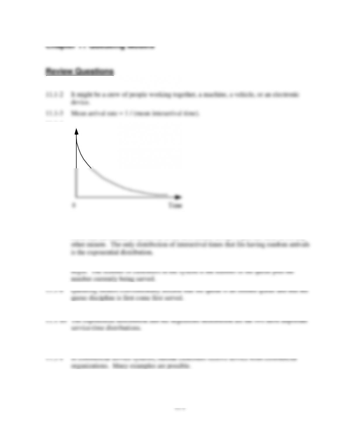
11.1-4
0 Time
11.1-5 The mean equals the standard deviation of the exponential distribution.
11.1-6 Having random arrivals means that arrival times are completely unpredictable in the
sense that the chance of an arrival in the next minute always is just the same as for any
11.1-7 The number of customers in the queue is the number of customers waiting for service to
11.1-9 Mean service time = 1 / (mean service rate).
11.1-11 The three parts of a label for queueing models provide information on the distribution of
service times, the number of servers, and the distribution of interarrival times.
11.2-2 In internal service systems, the customers receiving service are internal to the
organization. Many examples are possible.
11-2
11.2-3 In transportation service systems, either the customers or the servers are vehicles. Many
examples are possible.
11.3-2 Commercial service systems tend to place a greater importance on how long customers
typically have to wait.
11.3-3 L = expected number of customers in the system
11.3-4 A queueing system is in a steady state condition if it is in its normal condition after
11.3-8 Steady-state probabilities can also be used as measures of performance.
11.4-2 The issue is the increased number of complaints about intolerable waits for repairs on the
new copier.
11.4-4 Four alternative approaches have been suggested.
11.5-1
= expected number of arrivals per unit time
= expected number of service completions per unit time
11.5-2 (1) Interarrival times have an exponential distribution with a mean of (1/
); (2) service
11.5-5 The average waiting time until service begins is 6 hours.
Chapter 11 – Queueing Models
11.5-7 The M/G/1 model differs in the assumption about service time. In this model the service
times can have any probability distribution. It is not even necessary to determine the
11.5-9 Decreasing the standard deviation decreases Lq, L, W, and Wq.
11.6-1
=
/ (s
) which is the average fraction of time that individual servers are being utilized
serving customers.
11.6-3 Explicit formulas are available for all the measures of performance considered for the
M/M/1 model.
11.6-5 The M/M/s model has a great amount of variability in service times. The M/D/s model
has no variability.
11.7-2 With nonpreemptive priorities, once a server has begun serving a customer, the service
must be completed without interruption even if a higher priority customer arrives while
11.7-3 Except for using preemptive priorities, the assumptions are the same as for the M/M/1
model.
11.7-5
11.7-7 Two-person territories would be needed to reduce waiting times to acceptable levels.
11.8-1 Giving a relatively high utilization factor to the server provides surprisingly poor
measures of performance for the system.
11.8-3 Decreasing the variability of service times improves the performance of a single-server
queueing system substantially.

11-4
Chapter 11 – Queueing Models
11-5
11.8-5 Combining separate single-server queueing systems into one multiple-server queueing
system greatly improves the measures of performance.
11.8-7 Applying preemptive priorities improves the measures of performance for customers in
the top priority class even more than applying nonpreemptive priorities.
11.9-2 Making one’s own employees wait causes lost productivity, which results in lost profit
which is the waiting cost.
Problems
11.1 a) A hospital emergency room is a queueing system with patients as the customers and
care providers as the servers.
11.2
customer
server
a)
shoppers
checkout clerk
b)
fires
fire fighters / fire trucks
c)
cars
toll collectors
d)
bikes
bicycle repair people
e)
ships
longshoremen / docks
f)
machines
operator
g)
loads
handling equipment
h)
clogged pipes
plumber
i)
custom orders
customized process
j)
employees
secretary
11.3 a) True. The only distribution of interarrival times that fits having random arrivals is the
exponential distribution.
Chapter 11 – Queueing Models
11.4 a) False. Depending on the nature of the queueing system, the exponential distribution
can provide either a reasonable approximation or a gross distortion of the true service-
time distribution.
11.5 a) False. The queue is where customers wait before being served.
11.6 a) A bank is a queueing system with people as the customers, and tellers as the servers.
b) Wq = 1 minute
11.7 a) A parking lot is a queueing system for providing parking with cars as the customers,
and parking spaces as the servers. The service time is the amount of time a car spends
in a space. The queue capacity is 0.
b) L = 0P0 + 1P1 + 2P2 + 3P3 = 0(0.2) + 1(0.3) + 2(0.3) + 3(0.2) = 1.5 cars
Chapter 11 – Queueing Models
11-7
c) W = L/
= 2/4 = 0.5 hours = 30 minutes
before their haircut will begin.
11.9 The utilization factor
represents the fraction of time that the server is busy. The server
is busy except when there are zero people in the system. P0 is the probability of having 0
11.10 a) L =
/(
–
) = 30/(40–30) = 3 customers
W = 1/(
–
) = 1/(40–30) = 0.1 hours
P1 = (1–
)
= (1–0.75)(0.75) = 0.188
P2 = (1–
)
2 = (1–0.75)(0.75)2 = 0.141
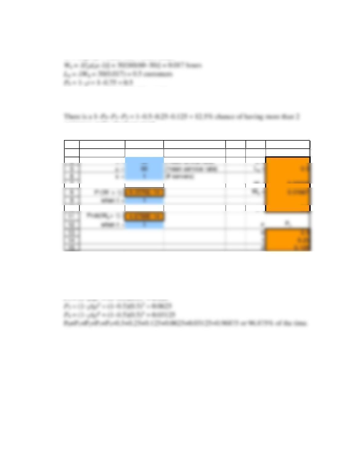
b) (M/M/1 model)
3
4
5
6
7
8
9
10
11
12
13
14
15
B C D E G H
Data Results
= 30 (mean arrival rate) L = 3
= 40 (mean service rate)
Lq = 2.25
s = 1 (# servers)
W = 0.1
Pr(W > t) = 4.54E-05
Wq = 0.075
when t = 1
= 0.75
Prob(Wq
> t) = 3.405E-05
when t = 1 n
Pn
0 0.25
1 0.1875
2 0.140625
Chapter 11 – Queueing Models
11-8
c) L =
/(
–
) = 30/(60–30) = 1 customer
W = 1/(
–
) = 1/(60–30) = 0.033 hours
P1 = (1–
)
= (1–0.75)(0.75) = 0.25
P2 = (1–
)
2 = (1–0.75)(0.75)2 = 0.125
customers at the checkout stand.
d) (M/M/s model)
3
4
5
6
7
8
9
10
11
12
13
14
15
B C D E G H
Data Results
= 30 (mean arrival rate) L = 1
= 60 (mean service rate)
Lq = 0.5
s = 1 (# servers)
W = 0.03333
Pr(W > t) = 9.3576E–14
Wq = 0.01667
when t = 1
= 0.5
Prob(Wq
> t) = 4.6788E–14
when t = 1 n
Pn
0 0.5
1 0.25
2 0.125
e) The manager should adopt the new approach of adding another person to bag the
groceries.
11.11 a) P0 = 1–
= 1–0.5 = 0.5
P1 = (1–
)
= (1–0.5)(0.5) = 0.25
2 = (1–0.5)(0.5)2 = 0.125
3 = (1–0.5)(0.5)3 = 0.0625
Chapter 11 – Queueing Models
11-9
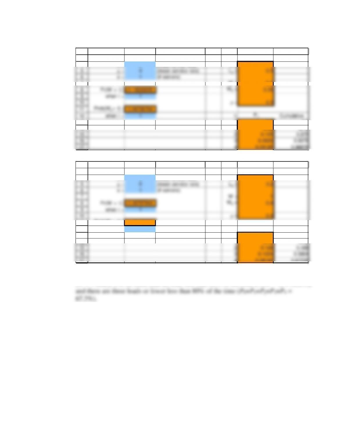
b) 96.875% of the time there are fewer than 4 in the system. (M/M/1 model)
3
4
5
6
7
8
9
10
11
12
13
14
15
16
17
B C D E G H I
Data Results
= 2 (mean arrival rate) L = 1
= 4 (mean service rate)
Lq = 0.5
s = 1 (# servers)
W = 0.5
Pr(W > t) = 0.13533528
Wq = 0.25
when t = 1
= 0.5
Prob(Wq
> t) = 0.06766764
when t = 1 n
PnCumulative
0 0.5 0.5
1 0.25 0.75
2 0.125 0.875
3 0.0625 0.9375
4 0.03125 0.96875
11.12 a) Tractor-trailer train (M/M/1 model):
3
4
5
6
7
8
9
10
11
12
13
14
15
16
17
B C D E G H I
Data Results
= 4 (mean arrival rate) L = 4
= 5 (mean service rate)
Lq = 3.2
s = 1 (# servers)
W = 1
Pr(W > t) = 0.36787944
Wq = 0.8
when t = 1
= 0.8
Prob(Wq
> t) = 0.29430355
when t = 1 n
PnCumulative
0 0.2 0.2
1 0.16 0.36
2 0.128 0.488
3 0.1024 0.5904
4 0.08192 0.67232
The train does not meet any of the criteria. The average time is more than half-an-hour
(W = 1 hour), it is no more than an hour less than 80% of the time (Pr(W > 1) = 36.8%),
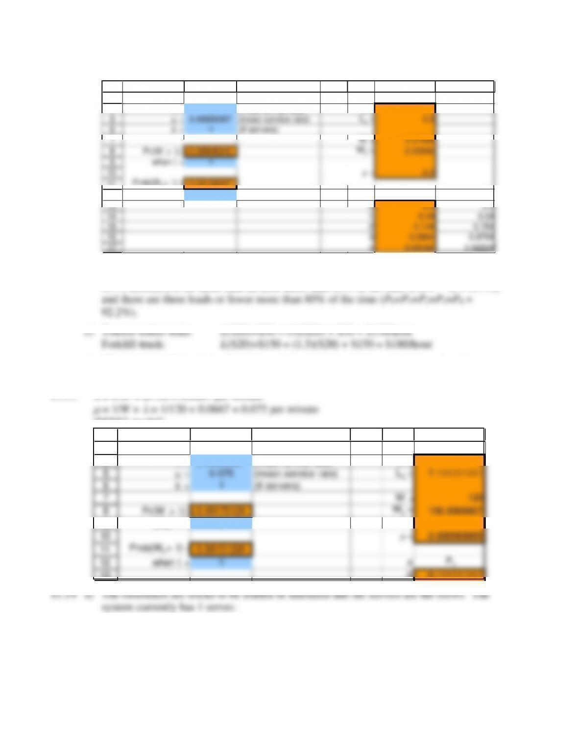
Chapter 11 – Queueing Models
b) Forklift truck (M/M/s model):
3
4
5
6
7
8
9
10
11
12
13
14
15
16
17
B C D E G H I
Data Results
= 4 (mean arrival rate) L = 1.5
= 6.66666667 (mean service rate)
Lq = 0.9
s = 1 (# servers)
W = 0.37500
Pr(W > t) = 0.06948345
Wq = 0.22500
when t = 1
= 0.6
Prob(Wq
> t) = 0.04169007
when t = 1 n
PnCumulative
0 0.4 0.4
1 0.24 0.64
2 0.144 0.784
3 0.0864 0.8704
4 0.05184 0.92224
The forklift truck meets all the criteria. The average time is less than half-an-hour (W =
0.375 hours), it is no more than an hour more than 80% of the time (Pr(W > 1) = 6.9%),
d) While the forklift truck has higher overall costs, it does a better job of meeting the
additional criteria.
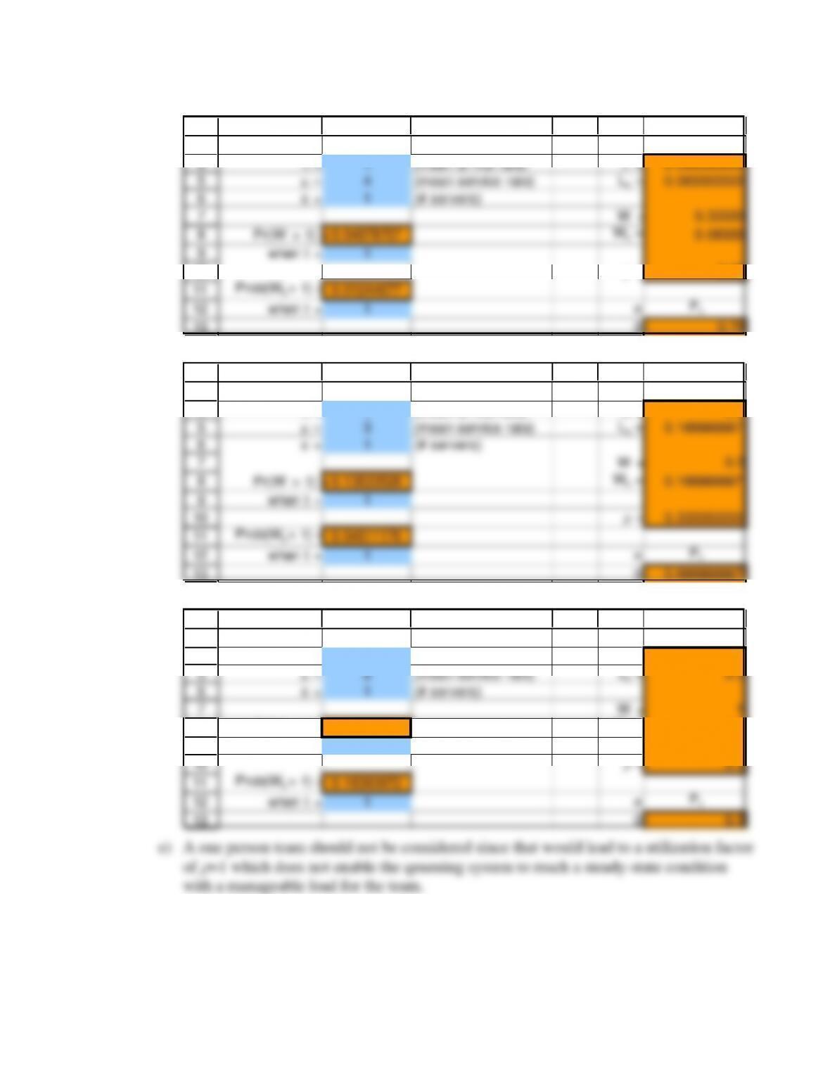
11.13
= L/W = 8/120 = 0.0667 per minute
(M/M/1 model)
3
4
5
6
7
8
9
10
11
12
13
B C D E G H
Data Results
= 0.06666667 (mean arrival rate) L = 8
= 0.075 (mean service rate)
Lq = 7.111111111
s = 1 (# servers)
W = 120
Pr(W > t) = 0.99170129
Wq = 106.6666667
when t = 1
= 0.888888889
Prob(Wq
> t) = 0.88151226
when t = 1 n
Pn
0 0.111111111
Chapter 11 – Queueing Models
11–11
b) 4 member crew (M/M/1 model):
3
4
5
6
7
8
9
10
11
12
13
B C D E G H
Data Results
= 1 (mean arrival rate) L = 0.333333333
= 4 (mean service rate)
Lq = 0.083333333
s = 1 (# servers)
W = 0.33333
Pr(W > t) = 0.04978707
Wq = 0.08333
when t = 1
= 0.25
Prob(Wq
> t) = 0.01244677
when t = 1 n
Pn
0 0.75
c) 3 member crew (M/M/1 model):
3
4
5
6
7
8
9
10
11
12
13
B C D E G H
Data Results
= 1 (mean arrival rate) L = 0.5
= 3 (mean service rate)
Lq = 0.166666667
s = 1 (# servers)
W = 0.5
Pr(W > t) = 0.13533528
Wq = 0.166666667
when t = 1
= 0.333333333
Prob(Wq
> t) = 0.04511176
when t = 1 n
Pn
0 0.666666667
d) 2 member crew (M/M/1 model):
3
4
5
6
7
8
9
10
11
12
13
B C D E G H
Data Results
= 1 (mean arrival rate) L = 1
= 2 (mean service rate)
Lq = 0.5
s = 1 (# servers)
W = 1
Pr(W > t) = 0.36787944
Wq = 0.5
when t = 1
= 0.5
Prob(Wq
> t) = 0.18393972
when t = 1 n
Pn
0 0.5
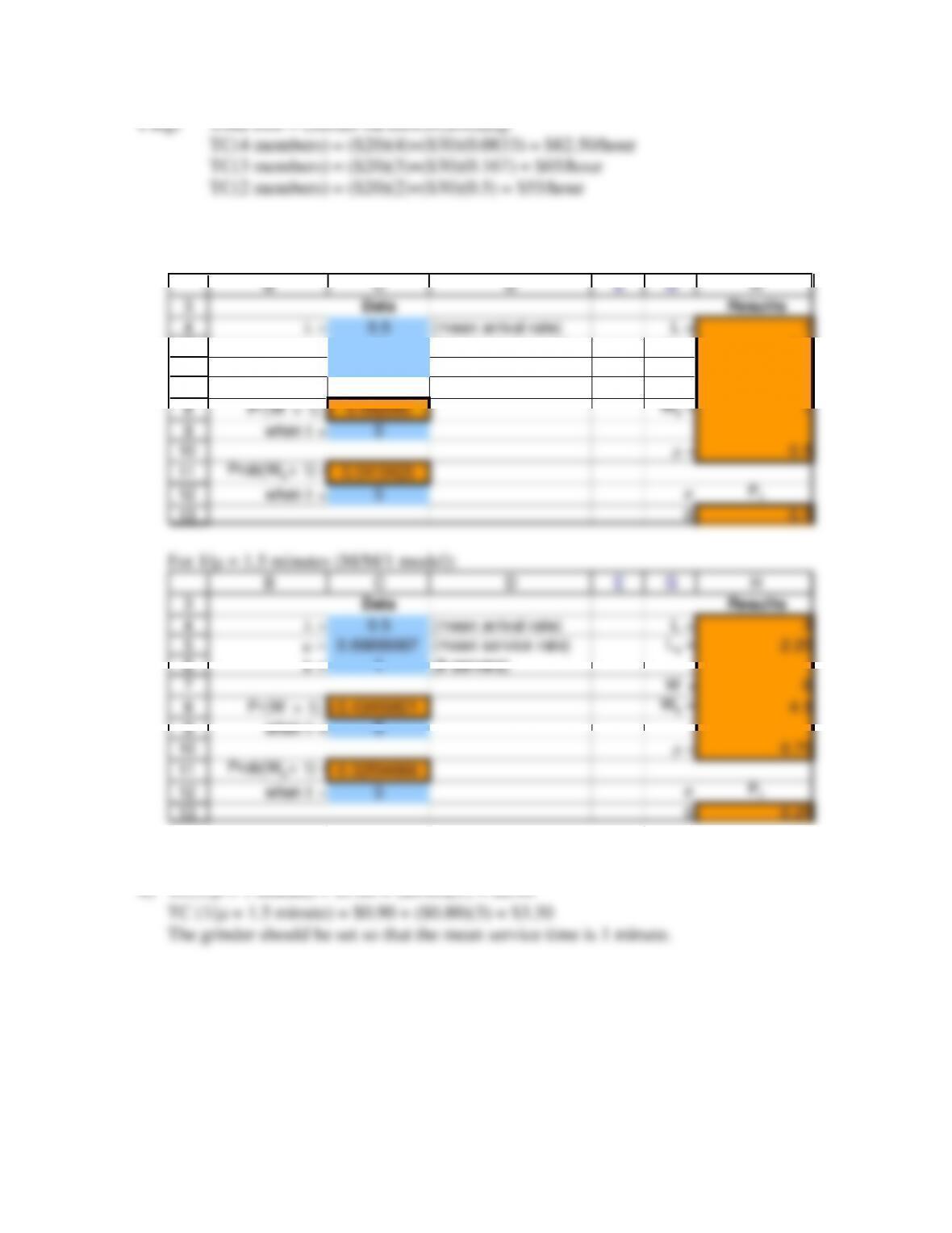
e) A one person team should not be considered since that would lead to a utilization factor
of
=1 which does not enable the qeueuing system to reach a steady-state condition
with a manageable load for the team.
Chapter 11 – Queueing Models
A crew of 2 people will minimize the expected total cost per hour.
11.15 a) 1/ = 1 minute (M/M/1 model):
3
4
5
6
7
8
9
10
11
12
13
B C D E G H
Data Results
= 0.5 (mean arrival rate) L = 1
= 1 (mean service rate)
Lq = 0.5
s = 1 (# servers)
W = 2
Pr(W > t) = 0.082085
Wq = 1
when t = 5
= 0.5
Prob(Wq
> t) = 0.0410425
when t = 5 n
Pn
0 0.5
For 1/ = 1.5 minutes (M/M/1 model):
3
4
5
6
7
8
9
10
11
12
13
B C D E G H
Data Results
= 0.5 (mean arrival rate) L = 3
= 0.66666667 (mean service rate)
Lq = 2.25
s = 1 (# servers)
W = 6
Pr(W > t) = 0.43459821
Wq = 4.5
when t = 5
= 0.75
Prob(Wq
> t) = 0.32594866
when t = 5 n
Pn
0 0.25
(1/
) = 2 minutes is not a feasible alternative since
=1.
Chapter 11 – Queueing Models
11–13
11.16 a) (M/M/1 model):
3
4
5
6
7
8
9
10
11
12
13
14
15
16
17
18
B C D E G H I
Data Results
= 10 (mean arrival rate) L = 1
= 20 (mean service rate)
Lq = 0.5
s = 1 (# servers)
W = 0.1
Pr(W > t) = 0.00673795
Wq = 0.05
when t = 0.5
= 0.5
Prob(Wq
> t) = 0.00336897
when t = 0.5 n
Pncumulative
0 0.5 0.5
1 0.25 0.75
2 0.125 0.875
3 0.0625 0.9375
4 0.03125 0.96875
5 0.015625 0.984375
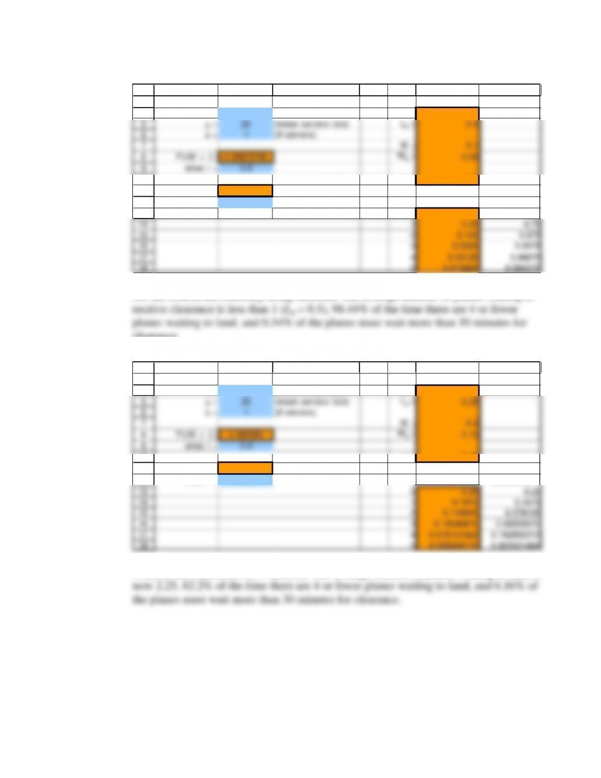
All the criteria are currently being satisfied. The average number of planes waiting to
clearance.
b) (M/M/1 model):
3
4
5
6
7
8
9
10
11
12
13
14
15
16
17
18
B C D E G H I
Data Results
= 15 (mean arrival rate) L = 3
= 20 (mean service rate)
Lq = 2.25
s = 1 (# servers)
W = 0.2
Pr(W > t) = 0.082085
Wq = 0.15
when t = 0.5
= 0.75
Prob(Wq
> t) = 0.06156375
when t = 0.5 n
Pncumulative
0 0.25 0.25
1 0.1875 0.4375
2 0.140625 0.578125
3 0.10546875 0.68359375
4 0.079101563 0.762695313
5 0.059326172 0.822021484
None of the criteria are now satisfied. The average number of planes waiting to land is
Chapter 11 – Queueing Models
c) (M/M/s model):
3
4
5
6
7
8
9
10
11
12
13
14
15
16
17
18
B C D E G H I
Data Results
= 25 (mean arrival rate) L = 2.051282051
= 20 (mean service rate)
Lq = 0.801282051
s = 2 (# servers)
W = 0.082051282
Pr(W > t) = 0.00102172
Wq = 0.032051282
when t = 0.5
= 0.625
Prob(Wq
> t) = 0.00026591
when t = 0.5 n
Pncumulative
0 0.230769231 0.230769231
1 0.288461538 0.519230769
2 0.180288462 0.699519231
3 0.112680288 0.812199519
4 0.07042518 0.8826247
5 0.044015738 0.926640437
In this case, the first and third criteria are satisfied but the second is not. The average
land.
11.17 Lq is unchanged and Wq is reduced by half. The arrival rate and service rate (and
variability) are all doubled. The system utilization is unchanged. The faster arrival rate
Chapter 11 – Queueing Models
11.18 a) M/G/1 Model:
3
4
5
6
7
8
9
10
11
12
13
14
15
16
17
18
19
20
21
22
B C D E F G
Data Results
= 0.2 (mean arrival rate) L = 2.5
= 4 (expected service time)
Lq = 1.7
= 1 (standard deviation)
s = 1 (# servers) W = 12.5
Wq = 8.5
= 0.8
P0 = 0.2
L
LqWWq
2.5 1.7 12.5 8.5
4 4 3.2 20 16
3 3.3 2.5 16.5 12.5
2 2.8 2 14 10
1 2.5 1.7 12.5 8.5
0 2.4 1.6 12 8
b) Lq is half with
= 0 therefore it is quite important to reduce the variability of the
service times.
c)
Lq
Change
4
3.2
3
2.5
0.7
largest reduction
2
2
0.5
1
1.7
0.3
0
1.6
0.1
smallest reduction
d) needs to be increased 0.05 (from 0.25 to 1/3.314 = 0.30) to achieve the same Lq (1.6).
3
6
7
B C D E F G
Data Results
= 4 (standard deviation)
s = 1 (# servers) W = 11.31595611
Wq = 8.001956109
Chapter 11 – Queueing Models
e) (M/G/1 Model):
3
4
5
6
7
8
9
10
11
12
13
14
15
16
17
18
19
20
21
22
23
24
25
26
27
B C D E F G
Data Results
= 0.2 (mean arrival rate) L = 4
= 4 (expected service time)
Lq = 3.2
= 4 (standard deviation)
s = 1 (# servers) W = 20
Wq = 16
= 0.8
P0 = 0.2
Lq
3.2
0.25 4 3.2
0.26 3.8462 2.6687
0.27 3.7037 2.2925
0.28 3.5714 2.0129
0.29 3.4483 1.7974
0.30 3.3333 1.6267
0.31 3.2258 1.4883
0.32 3.1250 1.3742
0.33 3.0303 1.2785
0.34 2.9412 1.1973
0.35 2.8571 1.1276
Chapter 11 – Queueing Models
f) (M/G/1 Model):
3
4
5
6
7
8
9
10
11
12
13
14
15
16
17
18
19
20
21
22
23
B C D E F G H
Data Resu lts
= 0.2 (mean arrival rate) L = 4
= 4 (expected service time)
Lq = 3.2
= 4 (standard deviation)
s = 1 (# servers) W = 20
Wq = 16
= 0.8
P0 = 0.2
3.2 4 3 2 1 0
0.22 4.5455 8.0655 6.5255 5.4255 4.7655 4.5455
0.24 4.1667 4.0033 3.1633 2.5633 2.2033 2.0833
0.26 3.8462 2.6687 2.0621 1.6287 1.3687 1.2821
0.28 3.5714 2.0129 1.5229 1.1729 0.9629 0.8929
0.30 3.3333 1.6267 1.2067 0.9067 0.7267 0.6667
Lq
11.19 a) False. When L increases, W also increases.
b) False. When and 2 are small, Lq is not necessarily small.
2/(1–
11.20 a) (M/G/1 Model):
3
4
5
6
7
8
B C D E F G
Data Resu lts
= 30 (mean arrival rate) L = 1.666666667
= 0.02083333 (expected service time)
Lq = 1.041666667
= 0.02083333 (standard deviation)
Chapter 11 – Queueing Models
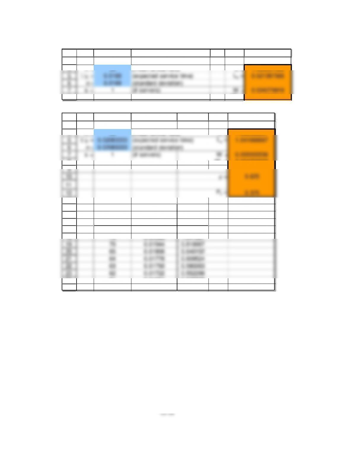
d) Marsha needs to reduce her service time to approximately 0.0169 hours = 61 seconds.
3
4
5
6
7
8
B C D E F G
Data Resu lts
= 30 (mean arrival rate) L = 1.028397566
= 0.0169 (expected service time)
Lq = 0.521397566
= 0.0169 (standard deviation)
s = 1 (# servers) W = 0.034279919
Wq = 0.017379919
e) (M/G/1 Model):
3
4
5
6
7
8
9
10
11
12
13
14
15
16
17
18
19
20
21
22
23
24
25
B C D E F G
Data Resu lts
= 30 (mean arrival rate) L = 1.666666667
= 0.02083333 (expected service time)
Lq = 1.041666667
= 0.02083333 (standard deviation)
s = 1 (# servers) W = 0.055555556
Wq = 0.034722222
= 0.625
P0 = 0.375
Service Service
Time Time
(seconds) (hours)
Lq
1.041667
75 0.02083 1.041667
70 0.01944 0.816667
65 0.01806 0.640152
64 0.01778 0.609524
63 0.01750 0.580263
62 0.01722 0.552299
61 0.01694 0.525565
60 0.01667 0.5
11–19
11.21 KeyCorp deploys queueing theory as part of its Service Excellence Management System
(SEMS) to improve productivity and service in its branches. The main objective of this
study is to enhance customer satisfaction by reducing wait times without increasing the
staffing costs. To do this, first a system that collects data about various phases of
customer transactions is developed. Then, a preliminary analysis is conducted to
new tellers was too costly and physically impossible. Alternatively, the bank could
achieve its goal by reducing the average service time. The investigation of the collected
data helped to identify potential improvements in service. Accordingly, customer
processing is reengineered, proficiency of tellers is improved and efficient schedules are
obtained. Heuristic algorithms are incorporated in the model to make it more realistic.
The model allowed KeyCorp to reduce the processing time by 53%. As a result of this,
the customer wait time has decreased and the percentage of customers who wait more
be used for more profitable investments. KeyCorp also gained more credibility by using a
systematic approach in making decisions. KeyCorp management, customers, employees
and shareholders all benefit from this study.
11.22 a) M/G/1 Model:
3
4
5
6
7
8
B C D E F G
Data Resu lts
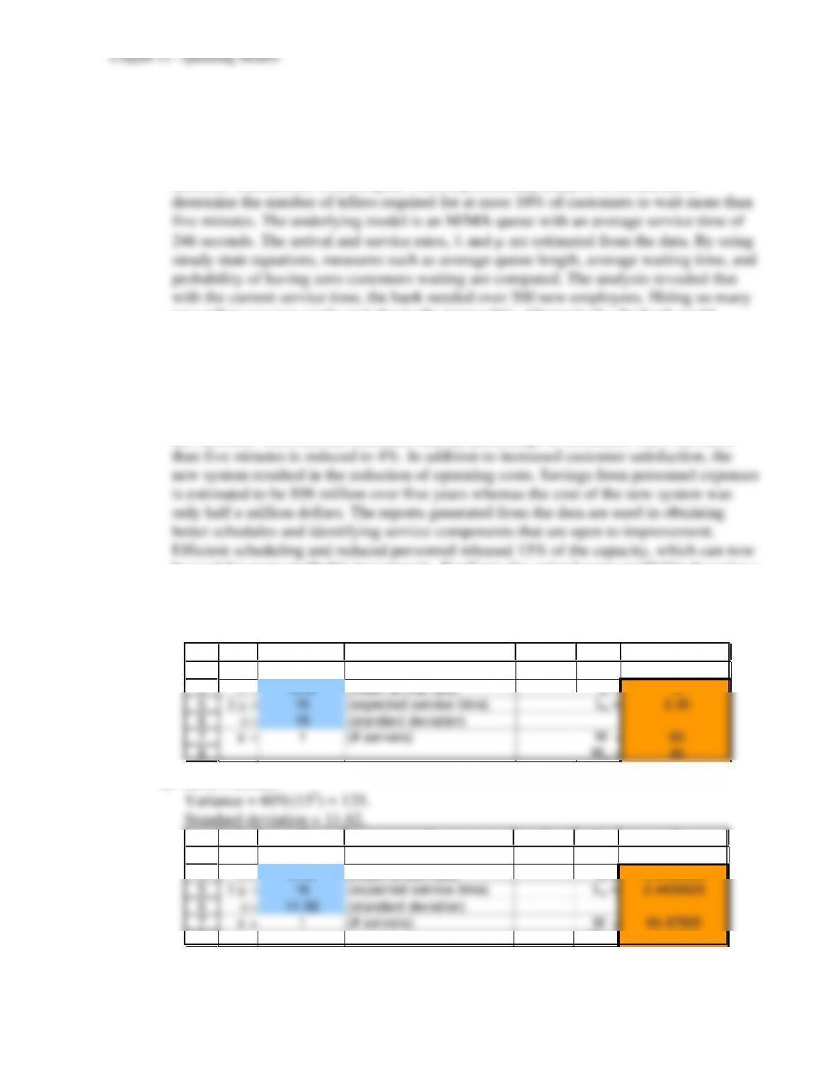
= 0.05 (mean arrival rate) L = 3
= 15 (expected service time)
Lq = 2.25
= 15 (standard deviation)
s = 1 (# servers) W = 60
Wq = 45
b) M/G/1 Model.
3
4
5
6
7
8
B C D E F G
Data Results
= 0.05 (mean arrival rate) L = 3.2439025
= 16 (expected service time)
Lq = 2.4439025
= 11.62 (standard deviation)
s = 1 (# servers) W = 64.87805
Wq = 48.87805

Chapter 11 – Queueing Models