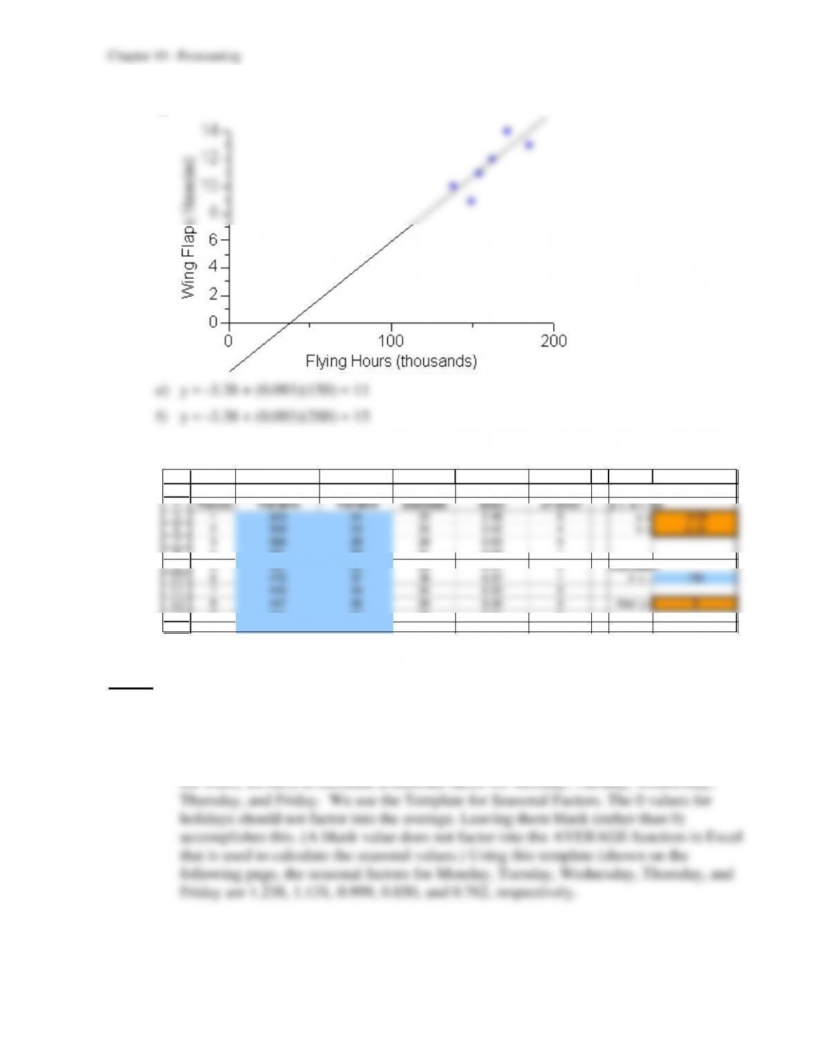
d)
10.41 Joe should use the linear regression line y = –9.95 + 0.10x to develop a forecast for jobs
(y) in terms of the number of permits issued (x).
3
4
5
6
7
8
9
10
11
12
13
14
B C D E F G H I J
Time Independent Dependent Estimation Square Linear Regression Lin e
Period Variable Variable Estimate Error of Error y = a + bx
1 323 24 22 2.48 6 a = –9.95
2 359 23 25 2.02 4 b = 0.10
3 396 28 29 0.63 0
4 421 32 31 0.93 1
5 457 34 35 0.57 0 Estimator
6 472 37 36 0.97 1 If x = 150
7 446 33 34 0.50 0
8 407 30 30 0.30 0 then y= 5
9 374 27 26 0.51 0
10 343 22 23 1.47 2
Case
10.1 a) We need to forecast the call volume for each day separately.
1) To obtain the seasonally adjusted call volume for the past 13 weeks, we first have to
determine the seasonal factors. Because call volumes follow seasonal patterns within

41
42
43
44
45
46
47
48
49
50
51
52
53
54
55
56
57
58
59
60
61
62
67
51 Tue
51 W ed
51 Thur 401
51 Fri 429
1
2
3
4
5
6
7
8
9
10
11
12
13
14
15
16
17
18
19
20
21
22
23
24
47 W ed 1,841
47 Thur
47 Fri
26
27
28
29
30
31
32
33
34
35
36
37
38
39
40
A B C D E F G
Template for Seasonal Factors
T rue
W eek Day Value Type of Seasonality
44 Mon 1,130 Daily
44 Tue 851
44 W ed 859
44 Thur 828 Estimate for
44 Fri 726 Day Season al Factor
45 Mon 1,085 Mon 1.238
45 Tue 1,042 Tue 1.131
45 W ed 892 W ed 0.999
45 Thur 840 Thur 0.850
45 Fri 799 Fri 0.762
46 Mon 1,303
46 Tue 1,121
46 W ed 1,003
46 Thur 1,113
46 Fri 1,005
47 Mon 2,652
47 Tue 2,825
48 Tue 1,507 1,025
48 W ed 989
48 Thur 990
48 Fri 1,084
49 Mon 1,260
49 Tue 1,134
49 W ed 941
49 Thur 847
49 Fri 714
50 Mon 1,002
50 Tue 847
50 W ed 922
50 Thur 842
50 Fri 784
51 Mon 823
10–35
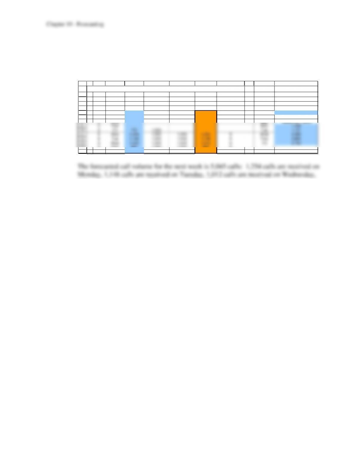
2) To forecast the call volume for the next week using the last-value forecasting
method, we need to use the Last Value with Seasonality template. To forecast the next
week, we need only start with the last Friday value since the Last Value method only
looks at the previous day.
1
2
3
4
5
6
7
8
9
10
11
12
13
14
15
A B C D E F G H I J K
Template for Last–Value Forecasting Method with Seasonality
Seasonally Season ally
T rue Adjusted Adjusted Actu al Forecastin g
W eek Day Value Value Forecast Forecast Error Type o f Seaso nality
5 Mon #N/A Daily
5 Tue #N/A #N/A
5 W ed #N/A #N/A Day Seasonal F actor
5 Thur #N/A #N/A Mon 1.238
5 Fri 772 1,013 #N/A Tue 1.131
6 Mon 1, 254 1,013 1,013 1,254 0 W ed 0.999
6 Tue 1,146 1,013 1,013 1,146 0 Thur 0.850
6 W ed 1,012 1,013 1,013 1,012 0 F ri 0. 762
6 Thur 860 1,012 1,013 860 0 1.000
6 Fri 771 1,012 1,012 771 0 1.000
860 calls are received on Thursday, and 771 calls are received on Friday.
49
50
51
52
53
55
56
57
58
59
60
61
63
64
65
66
68
73
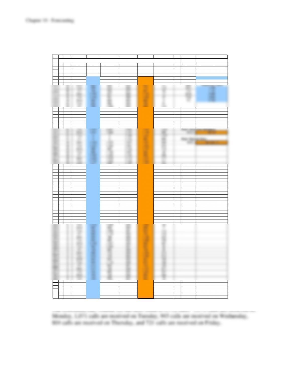
3) To forecast the call volume for the next week using the averaging forecasting
method, we need to use the Averaging with Seasonality template.
1
2
3
4
5
6
7
8
9
10
11
12
13
14
15
16
17
18
19
20
21
22
23
24
25
26
27
28
29
30
31
32
33
34
35
36
37
38
39
40
41
42
43
44
45
46
47
48
A B C D E F G H I J K
Template for Averaging Forecasting Method with Seasonality
Seasonally Season ally
T rue Adju sted Adjusted Actual Forecastin g
W eek Day Value Value Forecast F orecast Erro r Type o f Seasonality
44 Mon 1,130 913 Daily
44 Tue 851 752 913 1,033 182
44 W ed 859 860 833 832 27 Day Season al F actor
44 Thur 828 975 842 715 113 Mon 1.238
44 Fri 726 953 875 667 59 T ue 1.131
45 Mon 1,085 877 890 1,102 17 W ed 0.999
45 Tue 1,042 921 888 1,005 37 Thur 0.850
45 W ed 892 893 893 892 0 F ri 0.762
45 Thur 840 989 893 759 81 1.000
45 Fri 799 1,048 903 689 110 1.000
46 Mon 1,303 1,053 918 1,136 167 1.000
46 Tue 1,121 991 930 1,052 69 1.000
46 W ed 1, 003 1,004 935 934 69 1.000
46 Thur 1,113 1,310 941 799 314 1.000
46 Fri 1,005 1,319 967 737 268 1.000
47 Mon 2,652 2,143 990 1,226 1,426
47 Tue 2,825 2,497 1,062 1,202 1,623 Mean Absolute Deviation
47 W ed 1,841 1,842 1,147 1,146 695 MAD = 267.27
47 Thur 0 0 1,185 1,007 1,007
47 Fri 0 0 1,123 856 856 Mean Sq uare Error
48 Mon 1,949 1,575 1,067 1,321 628 MSE = 187, 916.17
48 Tue 1,507 1,332 1,091 1,234 273
48 W ed 989 990 1,102 1,101 112
48 Thur 990 1,165 1,097 932 58
48 Fri 1,084 1,422 1,100 838 246
49 Mon 1,260 1,018 1,113 1,377 117
49 Tue 1,134 1,002 1,109 1,255 121
49 W ed 941 942 1,105 1,104 163
49 Thur 847 997 1,099 934 87
49 Fri 714 937 1,096 835 121
50 Mon 1,002 810 1,091 1,350 348
50 Tue 847 749 1,081 1,224 377
50 W ed 922 923 1,071 1,070 148
50 Thur 842 991 1,067 906 64
50 Fri 784 1,029 1,064 811 27
51 Mon 823 665 1,063 1,316 493
51 Tue 0 0 1,052 1,191 1,191
51 W ed 0 0 1,024 1,023 1,023
51 Thur 401 472 997 847 446
51 Fri 429 563 983 750 321
52/1 Mon 1,209 977 973 1,204 5
52/1 T ue 830 734 973 1,101 271
52/1 W ed 0 0 967 967 967
10–37
4) To forecast the call volume for the next week using the moving-average forecasting
method, we need to use the Moving Averaging with Seasonality template. Since only
the past 5 days are used in the forecast, we start with Monday of the last week to
forecast through Friday of the next week.
1
2
3
4
5
6
7
8
9
10
11
12
13
14
15
16
A B C D E F G H I J K
Template for Moving–Average Forecasting Method with Seasonality
Season ally Seasonally
T rue Adjusted Adjusted Actual Forecasting Number o f previous
Week Day Value Valu e Forecast Forecast Error periods to consider
5 Mon 910 735 n = 5
5 Tue 754 666 #N/A
5 Wed 705 706 #N/A Type of Seasonality
5 Thur 729 858 #N/A Daily
5 Fri 772 1,013 #N/A
6 Mon 985 796 796 985 0 Day Seasonal Factor
6 Tue 914 808 808 914 0 Mon 1.238
6 Wed 835 836 836 835 0 Tue 1.131
6 Thur 732 862 862 732 0 Wed 0.999
6 Fri 658 863 863 658 0 T hur 0.850
7 Mon #N/A 833 1,031 Fri 0.762
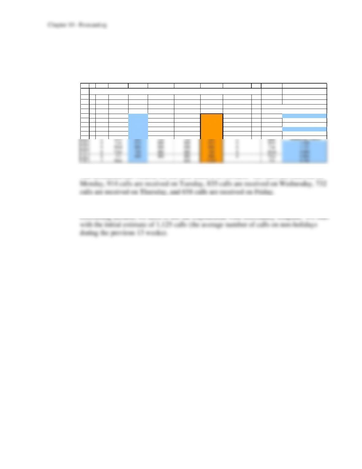
The forecasted call volume for the next week is 4,124 calls: 985 calls are received on
5) To forecast the call volume for the next week using the exponential smoothing
49
50
51
52
53
54
55
56
57
58
59
60
61
63
64
65
66
68
73
1
2
3
4
5
6
7
8
9
10
11
12
13
14
15
16
17
18
19
20
21
22
23
24
25
26
27
28
29
30
31
32
33
34
35
36
37
38
39
40
41
42
43
44
45
46
47
48
A B C D E F G H I J K
Template for Exponential Smoothing Forecasting Method with Seasonality
Seaso nally Seaso nally
T rue Adjusted Adjusted Actual Forecasting Smo othin g Constant
W eek Day Valu e Valu e F o recast F o recast Error = 0.1
44 Mon 1,130 913 1,025 1,269 139
44 Tue 851 752 1,014 1,147 296 Initial Estimate
44 W ed 859 860 988 987 128 Average = 1,025
44 Thur 828 975 975 828 0
44 Fri 726 953 975 743 17 T ype of Seaso n ality
45 Mon 1,085 877 973 1,204 119 Daily
45 Tue 1,042 921 963 1,089 47
45 W ed 892 893 959 958 66 Day Seasonal F actor
45 Thur 840 989 952 809 31 Mon 1.238
45 Fri 799 1,048 956 728 71 Tue 1.131
46 Mon 1,303 1,053 965 1,195 108 W ed 0.999
46 Tue 1,121 991 974 1,102 19 T hur 0.850
46 W ed 1,003 1,004 976 975 28 Fri 0.762
46 Thur 1,113 1,310 978 831 282 1.000
46 Fri 1,005 1,319 1,012 771 234 1.000
47 Mon 2,652 2,143 1,042 1,290 1,362 1.000
47 Tue 2,825 2,497 1,152 1,304 1,521 1.000
47 W ed 1,841 1,842 1,287 1, 286 555 1.000
47 Thur 0 0 1,342 1,140 1,140 1.000
47 Fri 0 0 1,208 921 921 1.000
48 Mon 1,949 1,575 1,087 1,346 603
48 Tue 1,507 1,332 1,136 1,285 222 Mean Absolute Deviation
48 W ed 989 990 1,156 1,155 166 MAD = 261.3
48 Thur 990 1,165 1,139 968 22
48 Fri 1,084 1,422 1,142 870 214 Mean Sq uare Error
49 Mon 1,260 1,018 1,170 1,448 188 MSE = 171,377.0
49 Tue 1,134 1,002 1,155 1,306 172
49 W ed 941 942 1,139 1,138 197
49 Thur 847 997 1,120 951 104
49 Fri 714 937 1,107 844 130
50 Mon 1,002 810 1,090 1,350 348
50 Tue 847 749 1,062 1,202 355
50 W ed 922 923 1,031 1,030 108
50 Thur 842 991 1,020 867 25
50 Fri 784 1,029 1,017 775 9
51 Mon 823 665 1,018 1,260 437
51 Tue 0 0 983 1,112 1,112
51 W ed 0 0 885 884 884
51 Thur 401 472 796 676 275
51 Fri 429 563 764 582 153
52/1 T ue 830 734 767 868 38
52/1 W ed 0 0 764 763 763
10–39
b) To obtain the mean absolute deviation for each forecasting method, we simply need to
subtract the true call volume from the forecasted call volume for each day in the sixth
1) The spreadsheet for the calculation of the mean absolute deviation for the last-value
forecasting method follows.
1
2
3
4
5
6
7
8
9
A B C D E F G H
Last Value
True Actual Forecast
Week Day Value Forecast Error
6 Monday 723 1,254 531
6 Tuesday 677 1,146 469
6 W ednesday 521 1,012 491
6 Thursday 571 860 289 Mean Abso lute Deviation
6 Friday 498 771 273 MAD = 410.6
This method is the least effective of the four methods because this method depends
heavily upon the average seasonality factors. If the average seasonality factors are not
the true seasonality factors for week 6, a large error will appear because the average
seasonality factors are used to transform the Friday call volume in week 5 to forecasts
for all call volumes in week 6. We calculated in part (a) that the call volume for Friday
10–40
2) The spreadsheet for the calculation of the mean absolute deviation for the averaging
forecasting method appears below.
1
2
3
4
5
6
7
8
9
A B C D E F G H
Averaging
True Actual F orecast
W eek Day Valu e F orecast Error
6 Monday 723 1,171 448
6 Tuesday 677 1,071 394
6 W ednesday 521 945 424
6 Thursday 571 804 233 Mean Absolute Deviation
6 Friday 498 721 223 MAD = 344.4
This method is the second-most effective of the four methods. Again, the reason lies in
the average seasonality factors. Applying the average seasonality factors to an average
call volume yields a much more accurate result than applying average seasonality
3)The spreadsheet for the calculation of the mean absolute deviation for the moving–
average forecasting method appears below.
1
2
3
4
5
6
7
8
9
A B C D E F G H
Moving Average
True Actual F orecast
W eek Day Valu e F orecast Error
6 Monday 723 985 262
6 Tuesday 677 914 237
6 W ednesday 521 835 314
6 Thursday 571 732 161 Mean Absolute Deviation
6 Friday 498 658 160 MAD = 226.8
This method is the most effective of the four methods because this method only uses
the average week 5 call volume to forecast the call volumes for week 6. Again,
10–41
4) The spreadsheet for the calculation of the mean absolute deviation for exponential
forecasting method follows.
1
2
3
4
5
6
7
8
9
A B C D E F G H
Exponential Smoothing
True Actual F orecast
W eek Day Valu e F orecast Error
6 Monday 723 1,074 351
6 Tuesday 677 982 305
6 W ednesday 521 867 346
6 Thursday 571 737 166 Mean Absolute Deviation
6 Friday 498 661 163 MAD = 266.2
This method is nearly as effective as the moving average. This method is a little more
effective than the averaging forecasting method because the smoothing constant causes
less weight to be placed on the call volumes in the earlier weeks.
c) This problem is simply a linear regression problem.
1) To find a mathematical relationship, we use the Linear Regression template. The
1
2
3
4
5
6
7
8
9
10
11
12
13
14
15
16
17
A B C D E F G H I J
Template for Linear Regression
In dependent Dependent Estimatio n Square Linear Regression Line
Week Variable Variable Estimate Error o f Error y = a + bx
44 612 2,052 2,038 13.84 192 a = 1,576
45 721 2,170 2,121 49.45 2,445 b = 0.76
46 693 2,779 2,099 679.61 461,872
47 540 2,334 1,984 350.27 122,690
48 1,386 2,514 2,623 109.26 11,938 Estimator
49 577 1,713 2,012 298.70 89,221 If x = 613
50 405 1,927 1,882 45.32 2,054
51 441 1,167 1,909 741.89 550,400 then y= 2,038.9
52/1 655 1,549 2,071 521.66 272,132
2 572 2,126 2,008 118.08 13,943
3 475 2,337 1,935 402.41 161,932
4 530 1,916 1,976 60.17 3,620
5 595 2,098 2,025 72.69 5,284

10–42
2) To forecast the week 6 call volume for the centralized call center, we simply input
the week 6 decentralized case volume for the value of x in the Estimator section of the
We then break this weekly call volume into daily call volume. We do this conversion
1
2
3
4
5
6
7
8
9
10
A B C
Week 6 Call Volume 3058
Daily Call Volume 611.6
Seasonal F orecasted
Day Factor Call Volume
Monday 1.238 757
Tuesday 1.131 692
Wednesday 0.999 611
Thursday 0.850 520
Friday 0.762 466
The forecasted call volume for week 6 is 3,046 calls: 757 calls are received on

10–43
3) To calculate the mean absolute deviation, we need to subtract the true call volume
from the forecasted call volume for each day in the sixth week. We then need to take
the absolute value of the five differences. Finally, we need to take the average of these
five absolute values to obtain the mean absolute deviation.
The spreadsheet for the calculation of the mean absolute deviation follows.
1
2
3
4
5
6
7
8
9
A B C D E F G H
Causal Forecasting
True Actual F orecast
W eek Day Valu e F orecast Error
6 Monday 723 757 34
6 Tuesday 677 692 15
6 W ednesday 521 611 90
6 Thursday 571 520 51 Mean Absolute Deviation
6 Friday 498 466 32 MAD = 44.4
This forecasting method is by far the most effective method. The centralized center
d) We would definitely recommend using the causal forecasting method implemented in
part (c) because it yields the lowest error. The causal method shows us that the call
volume trends remain relatively the same year after year. We had to convert between
case volumes and call volumes in part (c), however, and such a conversion introduces