e) Exponential-smoothing method with seasonality forecast = 22.
3
4
5
6
7
8
9
10
11
12
13
14
15
16
17
18
19
20
21
22
23
24
25
26
27
28
29
30
31
B C D E F G H I J K
Seasonally Seasonally
T ru e Adjusted Adjusted Actual Forecasting Smoothin g Constant
Year Quarter Value Value Forecast Forecast Error = 0.25
1 1 23 27 25 21 2
1 2 22 24 26 24 2Initial Estimate
1 3 31 26 25 30 1 Average = 25
1 4 26 25 25 26 0
2 1 19 23 25 21 2T ype o f Seaso nality
2 2 21 23 25 23 2 Q uarterly
2 3 27 23 24 29 2
2 4 24 23 24 25 1Q uarter Seasonal F actor
3 1 21 25 24 20 1 1 0.84
3 2 26 28 24 22 4 2 0.92
3 3 32 27 25 30 2 3 1.20
3 4 28 27 25 26 2 4 1.04
4 1 #N/A 26 22 1.000
4 2 #N/A #N/A 1.000
4 3 #N/A #N/A 1.000
4 4 #N/A #N/A 1.000
5 1 #N/A #N/A 1.000
5 2 #N/A #N/A 1.000
5 3 #N/A #N/A 1.000
5 4 #N/A #N/A 1.000
6 1 #N/A #N/A
6 2 #N/A #N/A Mean Absolu te Deviation
6 3 #N/A #N/A MAD = 1.66
6 4 #N/A #N/A
7 1 #N/A #N/A Mean Square Error
7 2 #N/A #N/A MSE = 3.56
f) Exponential-smoothing method with trend and seasonality forecast = 22.
3
4
5
6
7
8
9
10
11
12
13
14
15
16
17
18
19
20
21
22
23
24
25
26
27
28
29
30
31
32
33
B C D E F G H I J K L M
Season ally Seasonally
T ru e Adjusted L atest Estimated Adjusted Actual Forecasting Smo othing Constant
Year Quarter Value Value Trend T ren d Forecast Forecast Erro r = 0.25
1 1 23 27 025 21 2 = 0.25
1 2 22 24 1 0 26 24 2
1 3 31 26 0 0 25 30 1Initial Estimate
1 4 26 25 0 0 26 27 1 Average = 25
2 1 19 23 0 0 25 21 2 Trend = 0
2 2 21 23 -1 025 23 2
2 3 27 23 -1 024 29 2Typ e o f Seasonality
2 4 24 23 -1 023 24 0 Quart erly
3 1 21 25 0 0 23 19 2
3 2 26 28 0 0 23 21 5Q uarter Season al F acto r
3 3 32 27 1 0 25 29 3 1 0.84
3 4 28 27 1 0 25 26 2 2 0.92
4 1 #N/A 1 0 26 22 3 1.20
4 2 #N/A #N/A 4 1.04
4 3 #N/A #N/A 1.00
4 4 #N/A #N/A 1.00
5 1 #N/A #N/A 1.00
5 2 #N/A #N/A 1.00
5 3 #N/A #N/A 1.00
5 4 #N/A #N/A 1.00
6 1 #N/A #N/A 1.00
6 2 #N/A #N/A 1.00
6 3 #N/A #N/A
6 4 #N/A #N/A Mean Abso lu te Deviation
7 1 #N/A #N/A MAD = 1.78
7 2 #N/A #N/A
7 3 #N/A #N/A Mean Square Error
7 4 #N/A #N/A MSE = 4.42
g) The last-value method with seasonality has the lowest MAD and MSE value. Using this
method, the forecast for Q1 is 23 houses.
10–22
10.32 a)
Method
MAD
MSE
Last-value
3.07
12.89
Averaging
3.12
13.07
Moving-average
2.18
5.79
Exponential smoothing
2.34
9.31
b) The moving-average method with seasonality has the lowest MAD value. Using this
method, the forecast for January is 73 passengers.
3
4
5
6
7
8
9
10
11
12
13
14
15
16
17
18
19
20
21
22
23
24
25
26
27
28
29
B C D E F G H I J K
Season ally Season ally
T rue Adju sted Adjusted Actual Forecasting Number of previou s
Year Mo nth Value Value Forecast F orecast Error periods to con sider
1 Jan 68 76 n = 3
1 Feb 71 81 #N/A
1 Mar 66 73 #N/A Type of Seasonality
1 Apr 72 77 76 71 1 Monthly
1 May 77 80 77 74 3
1 June 85 78 77 84 1Month Season al Factor
1 July 94 80 79 92 2 Jan 0.90
1 Aug 96 83 80 91 5 Feb 0.88
1 Sep 80 82 81 78 2 Mar 0.91
1 Oct 73 80 82 75 2 Apr 0.93
1 Nov 84 80 82 86 2 May 0.96
1 Dec 89 82 81 87 2 June 1.09
2 Jan #N/A 81 73 July 1.17
2 Feb #N/A #N/A Aug 1.15
2 Mar #N/A #N/A Sep 0.97
2 Apr #N/A #N/A Oct 0.91
2 May #N/A #N/A Nov 1.05
2 June #N/A #N/A Dec 1.08
2 July #N/A #N/A
2 Aug #N/A #N/A Mean Abso lute Deviation
2 Sep #N/A #N/A MAD = 2.18
2 Oct #N/A #N/A
2 Nov #N/A #N/A Mean Square Error
2 Dec #N/A #N/A MSE = 5.79
10.33 a)
Method
MAD
MSE
Last-value
2.46
8.34
Averaging
7.06
74.73
Moving-average
2.79
9.68
Exponential smoothing
4.28
25.87
b) Exponential smoothing with trend and seasonality forecast = 94.
3
4
5
6
7
8
9
10
11
12
13
14
15
16
17
18
19
20
21
22
23
24
25
26
27
28
29
30
31
32
33
B C D E F G H I J K L M
Season ally Seasonally
T ru e Adjusted L atest Estimated Adjusted Actual Forecasting Smo othing Constant
Year Month Value Valu e Trend T ren d Forecast Forecast Error = 0.2
1 Jan 75 83 282 74 1 = 0.2
1 Feb 76 86 2 2 84 74 2
1 Mar 81 89 2 2 87 79 2Initial Estimate
1 Apr 84 90 3 2 90 83 1 Average = 80
1 May 85 89 2 2 92 88 3 Trend = 2
1 June 99 91 2 2 93 102 3
1 July 107 91 2 2 95 111 4 Type of Seasonality
1 Aug 108 94 1 2 96 110 2 Monthly
1 Sep 94 97 1 2 97 95 1
1 Oct 90 99 2 2 99 90 0Month Seasonal F actor
1 Nov 106 101 2 2 101 106 0 Jan 0.90
1 Dec 110 102 2 2 103 111 1 Feb 0.88
2 Jan #N/A 2 2 104 94 Mar 0.91
2 Feb #N/A #N/A Apr 0.93
2 Mar #N/A #N/A May 0.96
2 Apr #N/A #N/A June 1.09
2 May #N/A #N/A July 1.17
2 June #N/A #N/A Aug 1.15
2 July #N/A #N/A Sep 0.97
2 Aug #N/A #N/A Oct 0.91
2 Sep #N/A #N/A Nov 1.05
2 Oct #N/A #N/A Dec 1.08
2 Nov #N/A #N/A
2 Dec #N/A #N/A Mean Abso lu te Deviation
3 Jan #N/A #N/A MAD = 1.66
3 Feb #N/A #N/A
3 Mar #N/A #N/A Mean Square Error
3 Apr #N/A #N/A MSE = 4.21
MAD and MSE is lower here than all those found in part a.
c)
3
4
5
6
7
8
9
10
11
12
13
14
15
16
17
18
19
20
21
22
23
24
25
26
27
28
29
30
31
32
33
B C D E F G H I J K L M
Season ally Seasonally
T ru e Adjusted L atest Estimated Adjusted Actual Forecasting Smo othing Constant
Year Month Value Valu e Trend T ren d Forecast Forecast Error = 0.2
1 Jan 68 76 080 72 4 = 0.2
1 Feb 71 81 -1 079 69 2
1 Mar 66 73 0 0 79 72 6Initial Estimate
1 Apr 72 77 -1 077 72 0 Average = 80
1 May 77 80 0 0 77 74 3 Trend = 0
1 June 85 78 0 0 77 84 1
1 July 94 80 0 0 77 90 4T ype o f Seaso nali ty
1 Aug 96 83 0 0 78 89 7 Monthly
1 Sep 80 82 1 0 79 77 3
1 Oct 73 80 1 0 80 73 0Month Seasonal F actor
1 Nov 84 80 0 0 80 84 0 Jan 0.90
1 Dec 89 82 0 0 80 87 2 F eb 0.88
2 Jan 75 83 1 0 81 73 2 Mar 0.91
2 Feb 76 86 1 0 82 72 4 Apr 0.93
2 Mar 81 89 1 1 83 76 5 May 0.96
2 Apr 84 90 2 1 85 79 5 June 1.09
2 May 85 89 2 1 87 84 1 July 1.17
2 June 99 91 1 1 89 97 2 Aug 1.15
2 July 107 91 1 1 90 106 1 Sep 0.97
2 Aug 108 94 1 1 92 105 3 O ct 0.91
2 Sep 94 97 2 1 93 91 3 Nov 1.05
2 Oct 90 99 2 1 96 87 3 Dec 1.08
2 Nov 106 101 2 2 98 103 3
2 Dec 110 102 2 2 100 108 2 Mean Abso lu te Deviation
3 Jan #N/A 2 2 102 92 MAD = 2.74
3 Feb #N/A #N/A
3 Mar #N/A #N/A Mean Square Error
3 Apr #N/A #N/A MSE = 10.44
d) Exponential smoothing with trend should be used.

29
30
31
10.34 a)
3
4
5
6
7
8
9
10
11
12
13
14
15
16
17
18
19
20
21
22
23
24
25
26
27
28
B C D E F G
True
Year Month Value Type of Seasonality
1 Jan 352 Monthly
1 Feb 329
1 Mar 365
1 Apr 358 Estimate for
1 May 412 Month Seasonal Factor
1 June 446 Jan 0.81
1 July 420 Feb 0.81
1 Aug 471 Mar 0.88
1 Sep 355 Apr 0.92
1 Oct 312 May 1.02
1 Nov 567 June 1.11
1 Dec 533 July 1.02
2 Jan 317 Aug 1.19
2 Feb 331 Sep 0.81
2 Mar 344 Oct 0.76
2 Apr 386 Nov 1.44
2 May 423 Dec 1.26
2 June 472
2 July 415
2 Aug 492
2 Sep 340
2 Oct 301
2 Nov 629
2 Dec 505
10–25
b) Moving-average with seasonality:
3
4
5
6
7
8
9
10
11
12
13
14
15
16
17
18
19
20
21
22
23
24
25
26
27
28
29
30
B C D E F G H I J K
Seasonally Seasonally
T rue Adjusted Adju sted Actual Forecasting Number of previo us
Year Month Value Value Fo recast Forecast Error p eriods to con sider
1 Jan #N/A n = 3
1 Feb #N/A #N/A
1 Mar #N/A #N/A Type of Season ality
1 Apr #N/A #N/A Monthly
1 May #N/A #N/A
1 June #N/A #N/A Month Seasonal Factor
1 July #N/A #N/A Jan 0.81
1 Aug #N/A #N/A Feb 0.81
1 Sep #N/A #N/A Mar 0.88
1 Oct 335 440 #N/A Apr 0.92
1 Nov 594 413 #N/A May 1.02
1 Dec 527 420 #N/A June 1.11
2 Jan 364 450 424 343 21 July 1.02
2 Feb 343 425 428 345 2 Aug 1.19
2 Mar 391 446 432 378 13 Sep 0.81
2 Apr 437 474 440 406 31 Oct 0.76
2 May 458 451 448 456 2 Nov 1.44
2 June 494 447 457 505 11 Dec 1.26
2 July 468 460 457 465 3
2 Aug 555 467 453 538 17 Mean Absolute Deviation
2 Sep 387 480 458 369 18 MAD = 13.30
2 Oct 364 478 469 357 7
2 Nov 662 461 475 683 21 Mean Square Error
2 Dec 581 463 473 594 13 MSE = 249.09
3 Jan #N/A 467 378
c) Exponential smoothing with seasonality:
3
4
5
6
7
8
9
10
11
12
13
14
15
16
17
18
19
20
21
22
23
24
25
26
27
28
29
30
31
B C D E F G H I J K
Seasonally Seasonally
T ru e Adjusted Adjusted Actual Forecasting Smoothin g Constant
Year Month Value Value Forecast Forecast Error = 0.2
1 Jan 364 450 420 339 25
1 Feb 343 425 426 344 1 Initial Estimate
1 Mar 391 446 426 373 18 Average = 420
1 Apr 437 474 430 396 41
1 May 458 451 439 446 12 Type of Seasonality
1 June 494 447 441 488 6 Monthly
1 July 468 460 442 450 18
1 Aug 555 467 446 530 25 Month Seasonal Factor
1 Sep 387 480 450 363 24 Jan 0.81
1 Oct 364 478 456 347 17 Feb 0.81
1 Nov 662 461 461 662 0 Mar 0.88
1 Dec 581 463 461 579 2 Apr 0.92
2 Jan #N/A 461 373 May 1.02
2 Feb #N/A #N/A June 1.11
2 Mar #N/A #N/A July 1.02
2 Apr #N/A #N/A Aug 1.19
2 May #N/A #N/A Sep 0.81
2 June #N/A #N/A Oct 0.76
2 July #N/A #N/A Nov 1.44
2 Aug #N/A #N/A Dec 1.26
2 Sep #N/A #N/A
2 Oct #N/A #N/A Mean Absolu te Deviation
2 Nov #N/A #N/A MAD = 15.83
2 Dec #N/A #N/A
3 Jan #N/A #N/A Mean Sq uare Error
3 Feb #N/A #N/A MSE = 384.99
10–26
d) Exponential smoothing with trend and seasonality:
3
4
5
6
7
8
9
10
11
12
13
14
15
16
17
18
19
20
21
22
23
24
25
26
27
28
29
30
31
32
33
B C D E F G H I J K L M
Season ally Seasonally
T ru e Adjusted L atest Estimated Adjusted Actual Forecasting Smo othing Constant
Year Month Value Valu e Trend T ren d Forecast Forecast Error = 0.2
1 Jan 364 450 0 420 339 25 = 0.2
1 Feb 343 425 6 1 427 345 2
1 Mar 391 446 1 1 428 375 16 Initi al Estimate
1 Apr 437 474 5 2 433 399 38 Average = 420
1 May 458 451 10 3 445 452 6 Trend = 0
1 June 494 447 5 4 450 497 3
1 July 468 460 3 4 453 461 7 T ype o f Seaso nality
1 Aug 555 467 5 4 458 545 10 Monthly
1 Sep 387 480 6 4 464 374 13
1 Oct 364 478 7 5 472 359 5 Mo nth Season al F actor
1 Nov 662 461 6 5 479 688 26 Jan 0.81
1 Dec 581 463 2 4 479 602 21 F eb 0.81
2 Jan #N/A 1 4 480 388 Mar 0.88
2 Feb #N/A #N/A Apr 0.92
2 Mar #N/A #N/A May 1.02
2 Apr #N/A #N/A June 1.11
2 May #N/A #N/A July 1.02
2 June #N/A #N/A Aug 1.19
2 July #N/A #N/A Sep 0.81
2 Aug #N/A #N/A Oct 0.76
2 Sep #N/A #N/A Nov 1.44
2 Oct #N/A #N/A Dec 1.26
2 Nov #N/A #N/A
2 Dec #N/A #N/A Mean Abso lu te Deviation
3 Jan #N/A #N/A MAD = 14.26
3 Feb #N/A #N/A
3 Mar #N/A #N/A Mean Square Error
3 Apr #N/A #N/A MSE = 314.71
e) Moving average results in the best MAD value (13.30) and the best MSE value
(249.09).
f)
Month
Avg. Forecast
Forecasting
Error
January
341
23
February
345
2
March
375
16
April
400
37
May
451
7
June
497
3
July
459
9
August
537
18
September
369
18
October
354
10
November
677
15
December
592
12
g) Moving average performed better than the average of all three so it should be used next
year.
10–27
10.35 a)
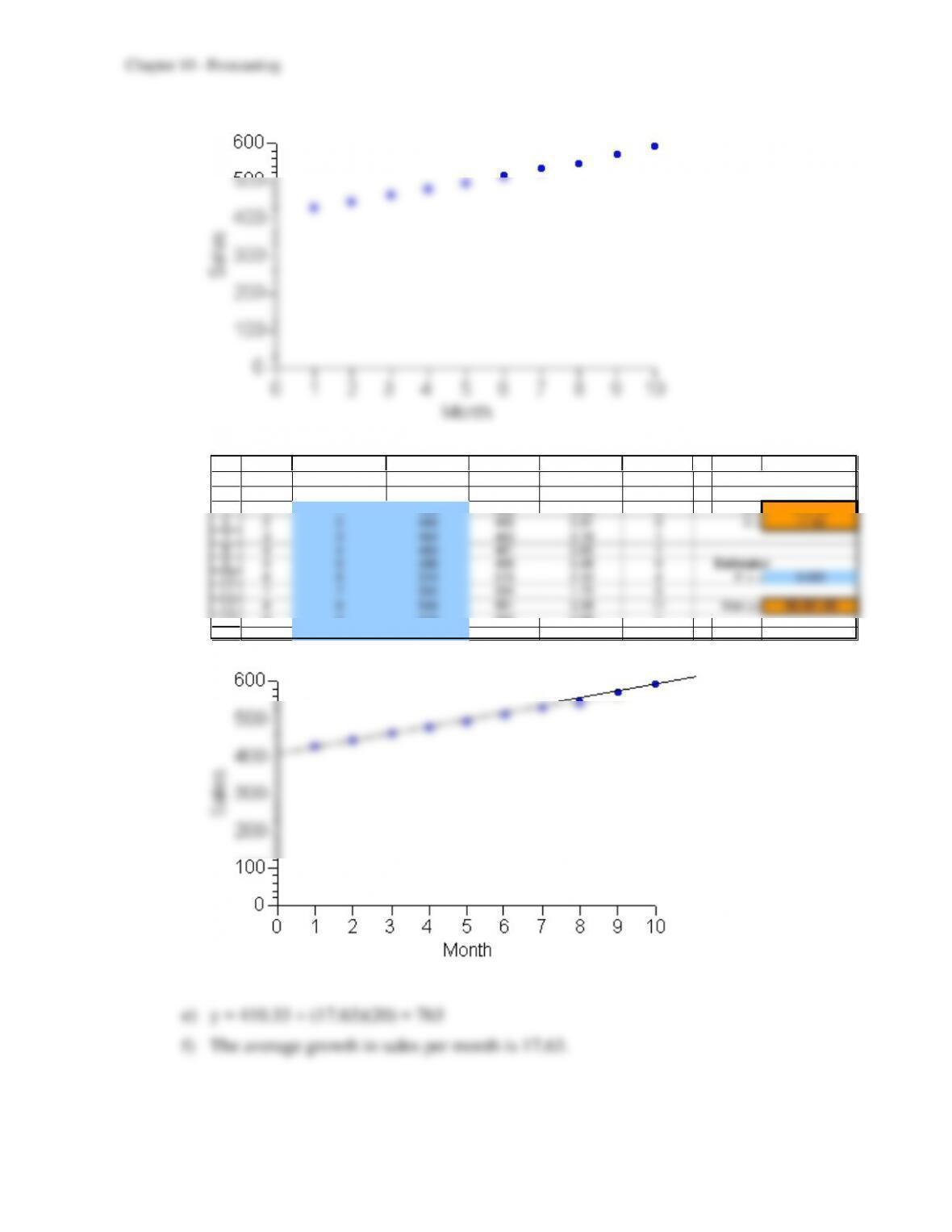
b) y = 410.33 + 17.63x
3
4
5
6
7
8
9
10
11
12
13
14
B C D E F G H I J
Time Independent Dependent Estimation Square Linear Regression L ine
Period Variable Variable Estimate Error of Error y = a + bx
1 1 430 428 2.04 4 a = 410.33
2 2 446 446 0.41 0 b = 17.63
3 3 464 463 0.78 1
4 4 480 481 0.85 1
5 5 498 498 0.48 0 Estimator
6 6 514 516 2.12 4 If x = 5,000
7 7 532 534 1.75 3
8 8 548 551 3.38 11 then y= 88,561.85
9 9 570 569 0.99 1
10 10 591 587 4.36 19
c)
d) y = 410.33 + (17.63)(11) = 604
10–28
10.36 a)
b)
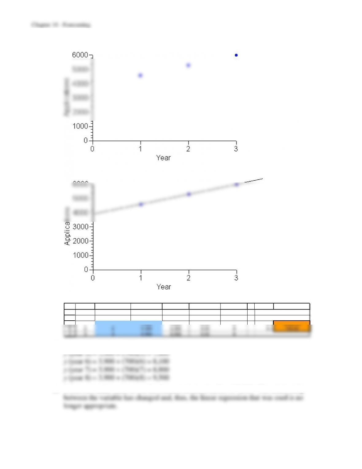
c) y = 3,900 + 700x
3
4
5
6
7
B C D E F G H I J
Time Independent Dependent Estimation Square L inear Regression Line
Period Variable Variable Estimate Error of Error y = a + bx
1 1 4,600 4,600 0.00 0 a = 3,900.00
2 2 5,300 5,300 0.00 0 b = 700.00
3 3 6,000 6,000 0.00 0
d) y (year 4) = 3,900 + (700)(4) = 6,700
e) It does not make sense to use the forecast obtained earlier of 9,500. The relationship
10–29
f)
3
4
5
6
7
8
9
10
11
12
B C D E F G H I J
Time Independent Dependent Estimation Square Linear Regression L ine
Perio d Variable Variable Estimate Error of Error y = a + bx
1 1 4,600 5,321 721.43 520,459 a = 5,229
2 2 5,300 5,414 114.29 13,061 b = 92.9
3 3 6,000 5,507 492.86 242,908
4 4 6,300 5,600 700.00 490,000
5 5 6,200 5,693 507.14 257,194 Estimator
6 6 5,600 5,786 185.71 34,490 If x = 8
7 7 5,200 5,879 678.57 460,459
8 then y= 5,971
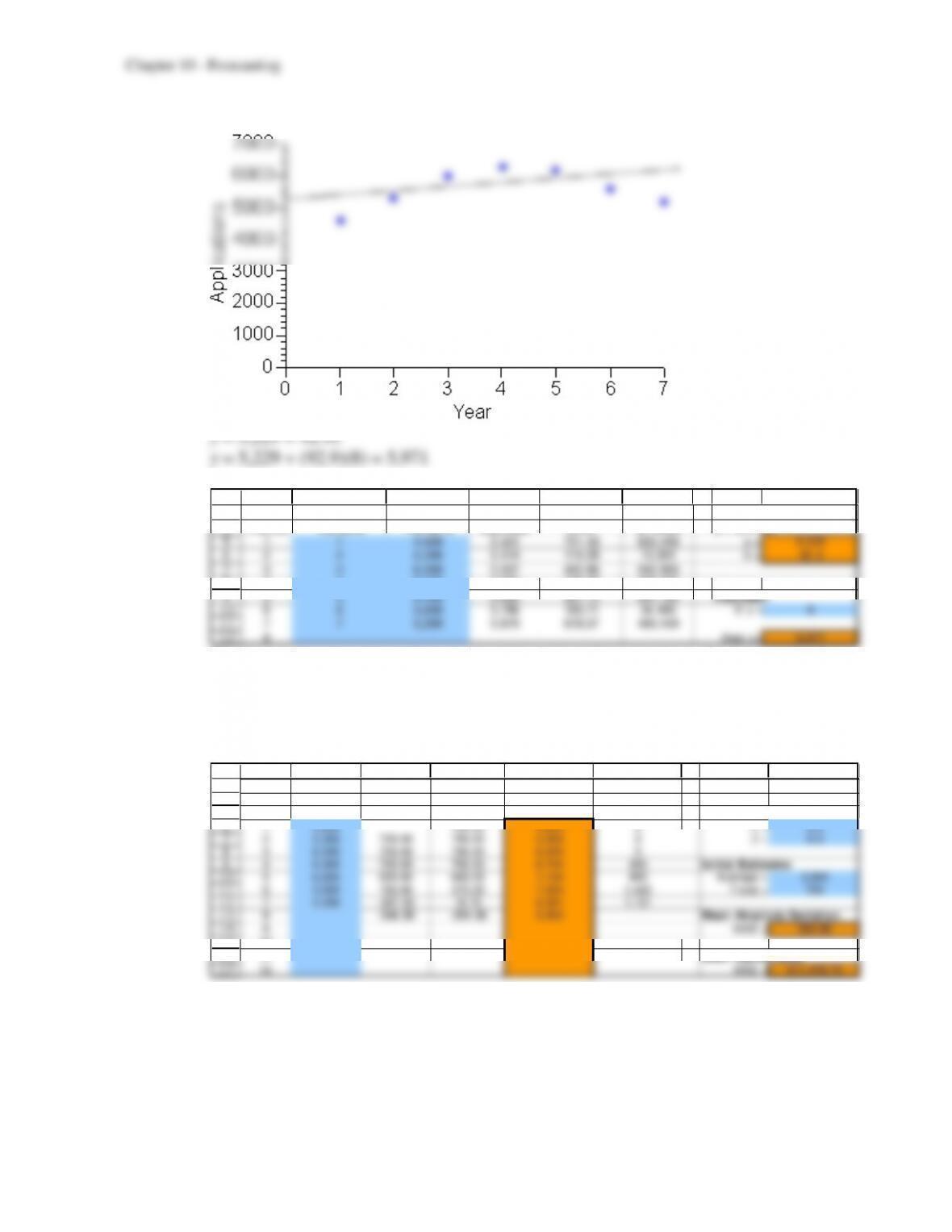
The linear regression line does not provide a close fit to the data. Consequently, the
forecast that it provides for year 8 is not likely to be accurate. It does not make sense to
continue to use a linear regression line when changing conditions cause a large shift in
the underlying trend in the data.
g)
3
4
5
6
7
8
9
10
11
12
13
14
15
16
17
B C D E F G H I J
Exponential
Time True Latest Estimated Smoothing Forecasting
Period Value Trend Trend Forecast Error Smoothing Constants
1 4,600 700.00 4,600 0 = 0.5
2 5,300 700.00 700.00 5,300 0 = 0.5
3 6,000 700.00 700.00 6,000 0
4 6,300 700.00 700.00 6,700 400 In itial Estimates
5 6,200 500.00 600.00 7,100 900 Average = 3,900
6 5,600 150.00 375.00 7,025 1,425 Trend = 700
7 5,200 -337.50 18.75 6,331 1,131
8 –546.88 -264.06 5,502 Mean Absolute Deviation
9#N/A MAD = 550.89
10 #N/A
11 #N/A Mean Square Error
12 #N/A MSE = 611,478.79
Causal forecasting takes all the data into account, even the data from before changing
conditions cause a shift. Exponential smoothing with trend adjusts to shifts in the
underlying trend by placing more emphasis on the recent data.
10–30
10.37 a)
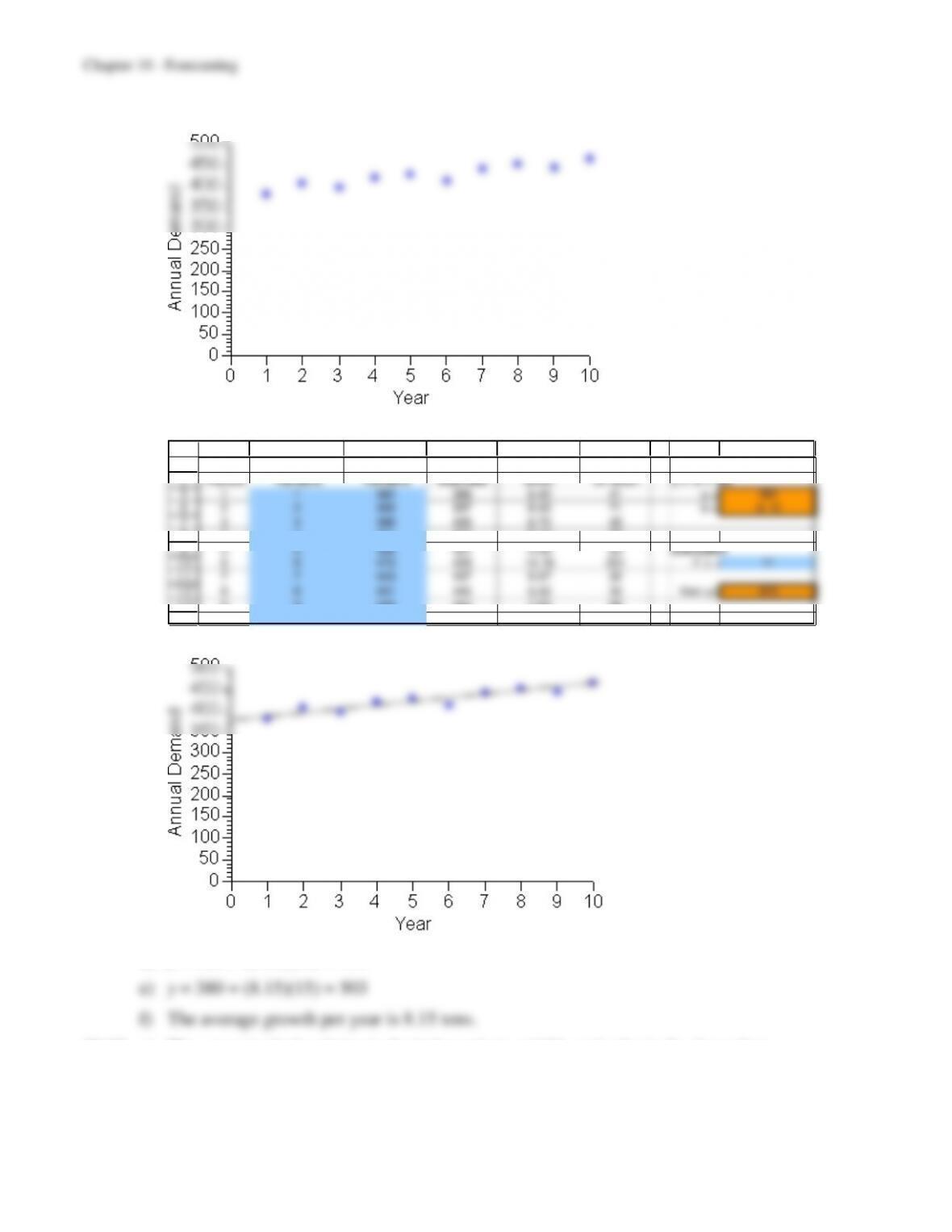
b) y = 380 + 8.15x
3
4
5
6
7
8
9
10
11
12
13
14
B C D E F G H I J
Time Independent Dependent Estimation Square L inear Regression Line
Period Variable Variable Estimate Error of Error y = a + bx
1 1 382 388 6.42 41 a = 380
2 2 405 397 8.43 71 b = 8.15
3 3 398 405 6.72 45
4 4 421 413 8.13 66
5 5 426 421 4.98 25 Estimator
6 6 415 429 14.18 201 If x = 11
7 7 443 437 5.67 32
8 8 451 445 5.52 30 then y= 470
9 9 446 454 7.63 58
10 10 464 462 2.22 5
c)
d) y = 380 + (8.15)(11) = 470
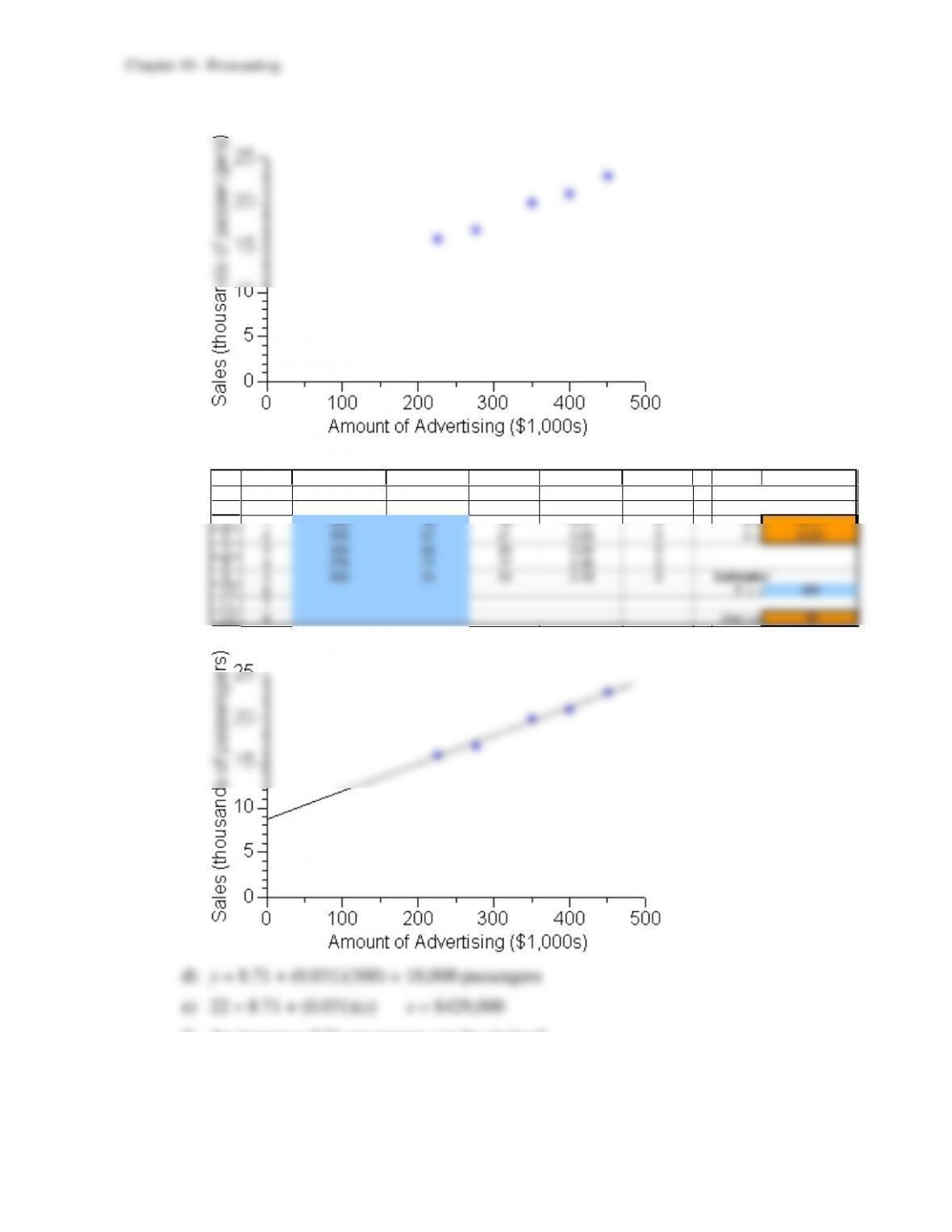
10.38 a) The amount of advertising is the independent variable and sales is the dependent
variable.
10–31
b)
c) y = 8.71 + 0.031x
3
4
5
6
7
8
9
10
11
12
B C D E F G H I J
Time Independent Dependent Estimation Square Linear Regression L ine
Perio d Variable Variable Estimate Error of Error y = a + bx
1 225 16 16 0.21 0 a = 8.71
2 400 21 21 0.29 0 b = 0.031
3 350 20 20 0.29 0
4 275 17 17 0.36 0
5 450 23 23 0.14 0 Estimator
6 If x = 300
7
8 then y= 18
f) An increase of 31 passengers can be attained.
10–32
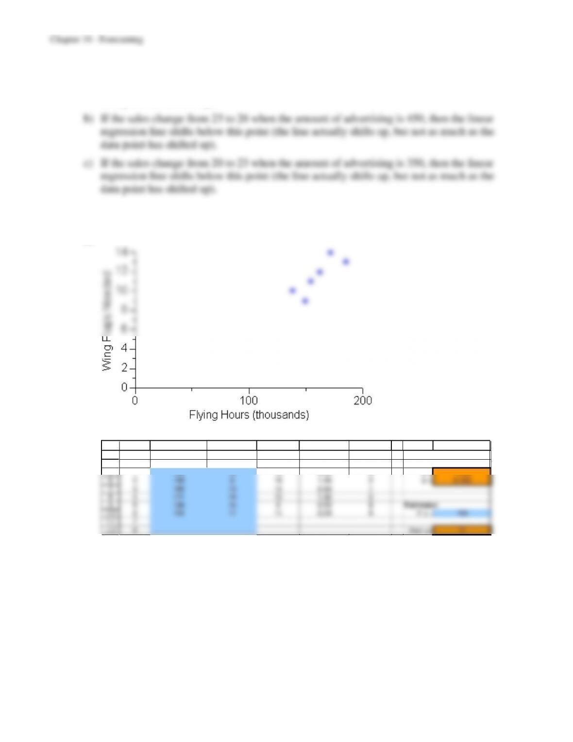
10.39 a) If the sales change from 16 to 19 when the amount of advertising is 225, then the linear
regression line shifts below this point (the line actually shifts up, but not as much as the
data point has shifted up).
10.40 a) The number of flying hours is the independent variable and the number of wing flaps
needed is the dependent variable.
b)
c) y = -3.38 + 0.093x
3
4
5
6
7
8
9
10
11
12
B C D E F G H I J
Time Independent Dependent Estimation Square Linear Regression L ine
Perio d Variable Variable Estimate Error of Error y = a + bx
1 162 12 12 0.30 0 a = –3.38
2 149 9 10 1.49 2 b = 0.093
3 185 13 14 0.84 1
4 171 14 13 1.46 2
5 138 10 9 0.53 0 Estimator
6 154 11 11 0.04 0 If x = 150
7
8 then y= 11