10-1
Chapter 10 Forecasting
Review Questions
10.1-1 The last-value forecasting method says simply to use the last period’s value as the forecast
conditions tend to remain so stable that even the earliestt periods are a reliable indicator of
the future.
10.1-3 The moving-average forecasting method uses the average of the previous n periods as a
forecast for the next period. This is a reasonable forecasting method when conditions tend
most recent periods. It gives the greatest weight to the last period and then progressively
smaller weights to older periods.
10.1-5 Exponential smoothing with trend adjusts exponential smoothing by also directly
considering any current upward or downward trend.
10.1-7 The mean absolute deviation (MAD) and the mean square error (MSE) are the two most
commonly used measures of accuracy of a forecasting method.
10.2-1 The company mails catalogs to its customers and prospective customers several times per
10.2-2 Customers who receive a busy signal or are on hold too long may not call back and
business may be lost. If too many agents are on duty there may be idle time, which wastes
money because of labor costs.
10.2-3 The current major frustration is that each time she has used her procedure for setting
10.2-4 Assume that each quarter’s call volume will be the same as for the preceding quarter,
except for adding 25% for quarter 4.
10-2
10.2-6 MSE is the mean square error. Its formula is (Sum of square of forecasting errors) /
(Number of forecasts).
10.3-1 In general, the seasonal factor for any period of a year measures how that period compares
to the overall average for an entire year.
10.3-4 The last-value forecasting method sometimes is called the naive method because
statisticians consider it naive to use just a sample size of one when additional relevant data
are available.
10.3-6 Rather than using old data that may no longer be relevant, this method averages the data
for only the most recent periods.
10.3-8 A small value is appropriate if conditions are remaining relatively stable. A larger value is
needed if significant changes in the conditions are occurring relatively frequently.
10.3-10 The one big factor that drives total sales up or down is whether there are any hot new
products being offered.
10.4-1 The next value that will occur in a time series is a random variable.
10.4-2 The goal of time series forecasting methods is to estimate the mean of the underlying
probability distribution of the next value of the time series as closely as possible.
10.4-3 No, the probability distribution is not the same for every quarter.
10.4-5 A time series is said to be stable if its underlying probability distribution usually remains
the same from one time period to the next. A time series is unstable if both frequent and
10-3
10.5-1 Causal forecasting obtains a forecast of the quantity of interest by relating it directly to
one or more other quantities that drive the quantity of interest.
10.5-2 The dependent variable is call volume and the independent variable is sales.
times the variable, added on the right-hand side for each of these variables.
10.5-5 The procedure used to obtain a and b is called the method of least squares.
10.6-1 Statistical forecasting methods cannot be used if no data are available, or if the data are
not representative of current conditions.
10.6-3 The jury of executive opinion method involves a small group of high-level managers who
pool their best judgment to collectively make a forecast rather than just the opinion of a
single manager.
10.6-5 A consumer market survey is helpful for designing new products and then in developing
the initial forecasts of their sales. It is also helpful for planning a marketing campaign.
Problems
10.1 a) Forecast = last value = 39
d) It appears as if demand is rising so the average forecasting method seems inappropriate
because it uses older, out-of-date data.
d) The averaging method seems best since all five months of data are relevant in
determining the forecast of sales for next month and the data appears relatively stable.
10-4
10.3
Quarter
Forecast
True Value
Error
1
327
345
18
2
332
317
15
3
328
336
8
4
330
311
19
MAD = (Sum of forecasting errors) / (Number of forecasts)
10.4 a) Method 1 MAD = (258 + 499 + 560 + 809 + 609) / 5 = 2,735 / 5 = 547
Method 2 gives a lower MAD and MSE.
b) She can use the older data to calculate more forecasting errors and compare MAD for a
10.5 At the time this article was written, L.L. Bean generated most of its sales through orders
taken at the company’s call center. (A separate call center is used for inquiries to the
company.) Since the sales volume is highly seasonal and even varies by day of the week,
The new forecasting system performed very well. Avoiding understaffing of the call
centers provided better customer service. Avoiding overstaffing avoided wasted personnel
10-5
10.6 a)
Quarter
Call Volume
Seasonal Factor
1
6809
6,089 / 7,027 = 0.97
2
6465
6,465 / 7,027 = 0.92
3
6569
6,569 / 7,027 = 0.93
4
8266
8,266 / 7,027 = 1.18
b)
Quarter
Seasonal
Factor
Actual
Call
Volume
Seasonally Adjusted
Call Volume
1
0.97
7,257
7,257 / 0.97 = 7,481
2
0.92
7,064
7,064 / 0.92 = 7,678
3
0.93
7,784
7,784 / 0.93 = 8,370
4
1.18
8,724
8,724 / 1.18 = 7,393
c)
Quarter
Two-Year
Average
Seasonal Factor
1
7,033
7,033 / 7,367 = 0.95
2
6,765
6,765 / 7,367 = 0.92
3
7,177
7,177 / 7,367 = 0.97
4
8,495
8,495 / 7,367 = 1.15
d)
Quarter
Seasonal
Factor
Actual
Call
Volume
Seasonally Adjusted
Call Volume
1
0.95
6992
6,992 / 0.95 = 7,360
2
0.92
6822
6,822 / 0.92 = 7,415
3
0.97
7949
7,949 / 0.97 = 8,195
4
1.15
9650
9,650 / 1.15 = 8,391
10.7 a)
Quarter
Unemployment Rate
Seasonal Factor
1
6.2%
6.2% / 6.3% = 0.98
2
6.0%
6.0% / 6.3% = 0.95
3
7.5%
7.5% / 6.3% = 1.19
4
5.5%
5.5% / 6.3% = 0.87
10-6
b)
Quarter
Seasonal
Factor
Actual
Unemployment Rate
Seasonally Adjusted
Call Volume
1
0.98
7.8%
7.8% / 0.98 = 8.0%
2
0.95
7.4%
7.4% / 0.95 = 7.8%
3
1.19
8.7%
8.7% / 1.19 = 7.3%
4
0.87
6.1%
6.1% / 0.87 = 7.0%
This progression indicates that the state’s economy is improving with the
unemployment rate decreasing from 8% to 7% (seasonally adjusted) over the four
quarters.
10.8 a)
Quarter
Three-Year Average
Seasonal Factor
1
21
21 /25 = 0.84
2
23
23 /25 = 0.92
3
30
30 / 25 = 1.20
4
26
26 / 25 = 1.04
b) Seasonally adjusted value for Y3(Q4) = 28 / 1.04 = 27,
c) Y4(Q1) = 23 as shown in part b
Seasonally adjusted value for Y4(Q2) = 25 / 0.92 = 27
Seasonally adjusted value for Y4(Q3) = 33/1.20 = 27
d)
Quarter
Seasonal
Factor
Average
House Sales
Seasonally Adjusted
Forecast
1
0.84
25
(25)(0.84) = 21
2
0.92
25
(25)(0.92) = 23
3
1.20
25
(25)(1.20) = 30
4
1.04
25
(25)(1.04) = 26
10.9 Forecast = 2,083 – (1,945 / 4) + (1,977 / 4) = 2,091
10-7
10.12 Forecast(
) =
(last value) + (1 –
)(last forecast)
10.13 Forecast(
) =
(last value) + (1 –
)(last forecast)
Forecast(0.1) = (0.1)(1,973) + (1 – 0.1)(2,083) = 2,072
10.14 This study uses integer programming to model employee scheduling problem of Taco Bell
restaurants. In this integer program, the decision variables correspond to the number of
employees scheduled to start working at time t and to work for s time units. The objective
is to minimize the total payroll for the scheduling horizon. At any point in time, the labor
10.15 a) Forecast(year 1) = initial estimate = 5000
b) MAD = (400 + 400 + 1,000) / 3 = 600
10.16 Forecast =
(last value) + (1 –
)(last forecast) + Estimated trend
Estimated trend =
(Latest trend) + (1 –
)(Latest estimate of trend)
Forecast (year 3) = (0.25)(5,300) + (1 – 0.25)(5,300) + (0.25)[(0.25)(5,300 – 4,600)
+ (1 – 0.25)(5,300 – 4,600)]+(1 – 0.25)(700) = 6,000
10.17 Forecast =
(last value) + (1 –
)(last forecast) + Estimated trend
Estimated trend =
(Latest trend) + (1 –
)(Latest estimate of trend)
10.18 Forecast =
(last value) + (1 –
)(last forecast) + Estimated trend
Estimated trend =
(Latest trend) + (1 –
)(Latest estimate of trend)
10.19 a) Since sales are relatively stable, the averaging method would be appropriate for
forecasting future sales. This method uses a larger sample size than the last-value
b) Last-Value Method:
3
4
5
6
7
8
9
10
11
12
13
14
15
16
17
B C D E F G H
Time True Last-Value F orecasting
Period Value Fo recast Error Mean Absolute Deviation
123 MAD = 5.2
224 23 1
322 24 2Mean Sq uare Error
428 22 6 MSE = 30.6
522 28 6
627 22 5
720 27 7
826 20 6
921 26 5
10 29 21 8
11 23 29 6
12 28 23 5
13 28
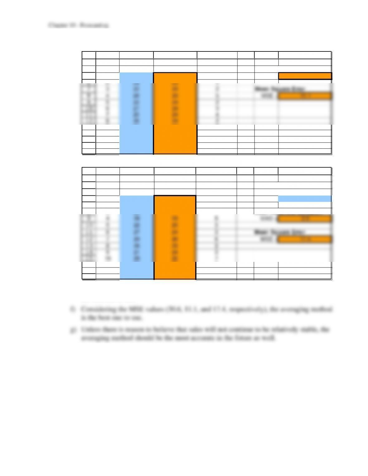
c) Averaging Method:
3
4
5
6
7
8
9
10
11
12
13
14
15
16
17
B C D E F G H
Time True Averaging Forecasting
Period Valu e Forecast Error Mean Abso lute Deviatio n
123 MAD = 3.0
224 23 1
322 24 2Mean Sq u are Error
428 23 5 MSE = 11.1
522 24 2
627 24 3
720 24 4
826 24 2
921 24 3
10 29 24 5
11 23 24 1
12 28 24 4
13 24
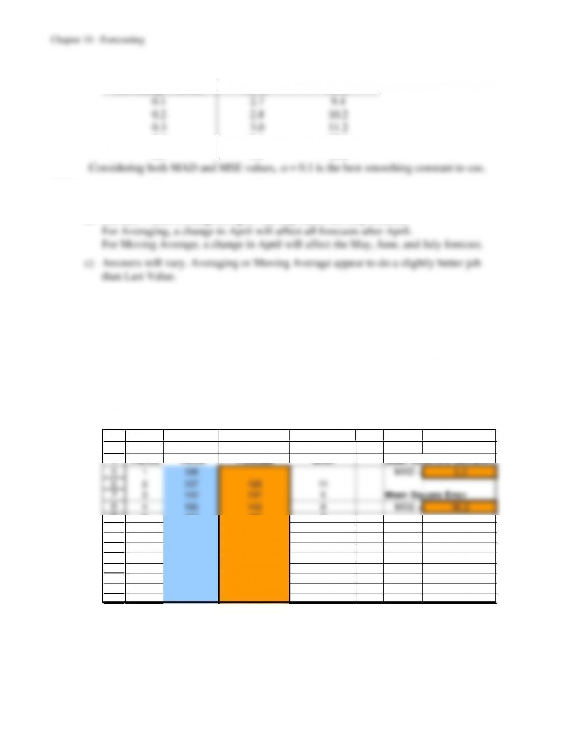
d) Moving Average Method (n = 3):
3
4
5
6
7
8
9
10
11
12
13
14
15
16
17
18
B C D E F G H
Mo ving
Time True Average Forecastin g Number o f previous
Period Valu e Forecast Error perio ds to consider
123 n= 3
224 #N/A
322 #N/A Mean Absolute Deviation
428 23 5 MAD = 3.9
522 25 3
627 24 3Mean Sq uare Error
720 26 6 MSE = 17.4
826 23 3
921 24 3
10 29 22 7
11 23 25 2
12 28 24 4
13 27
e) Considering the MAD values (5.2, 3.0, and 3.9, respectively), the averaging method is
the best one to use.
10.20 Using the template for exponential smoothing, with an initial estimate of 24, the following
forecast errors were obtained for various values of the smoothing constant
:
10–10
Smoothing Constant
MAD
MSE
0.1
2.7
9.4
0.2
2.8
10.2
0.3
3.0
11.2
0.4
3.1
12.4
0.5
3.3
13.8
10.21 a) Answers will vary. Averaging or Moving Average appear to do a better job than Last
Value.
b) For Last Value, a change in April will only affect the May forecast.
d) Answers will vary. Averaging or Moving Average appear to do a slightly better job
than Last Value.
10.22 a) Since the sales level is shifting significantly from month to month, and there is no
consistent trend, the last-value method seems like it will perform well. The averaging
method will not do as well because it places too much weight on old data. The moving–
average method will be better than the averaging method but will lag any short-term
trends. The exponential smoothing method will also lag trends by placing too much
weight on old data. Exponential smoothing with trend will likely not do well because
the trend is not consistent.
b) Last-value method:
3
4
5
6
7
8
9
10
11
12
13
14
15
16
17
B C D E F G H
Time True Last-Value Forecasting
Period Value Forecast Error Mean Absolute Deviation
1 126 MAD = 5.3
2 137 126 11
3 142 137 5 Mean Square Error
4 150 142 8 MSE = 36.2
5 153 150 3
6 154 153 1
7 148 154 6
8 145 148 3
9 147 145 2
10 151 147 4
11 159 151 8
12 166 159 7
13 166
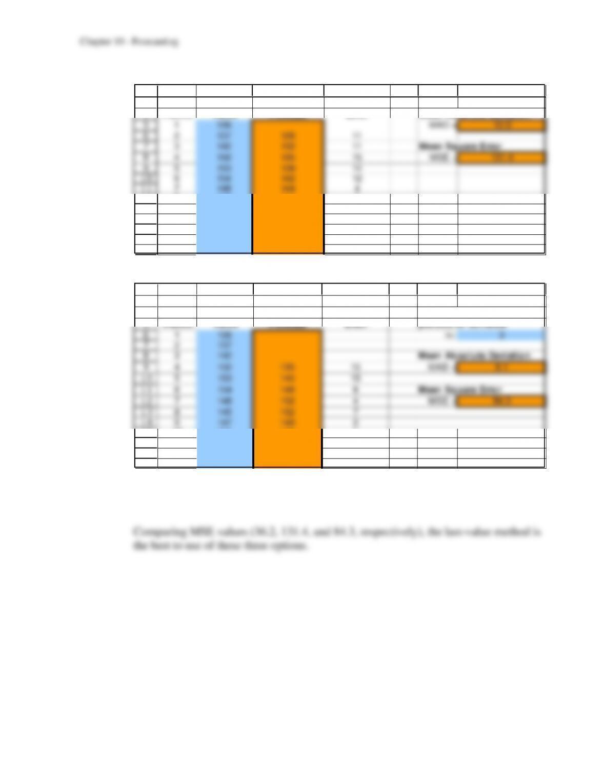
Averaging method:
3
4
5
6
7
8
9
10
11
12
13
14
15
16
17
B C D E F G H
Time True Averaging Forecasting
Period Valu e Forecast Error Mean Abso lute Deviatio n
1 126 MAD = 10.0
2 137 126 11
3 142 132 11 Mean Sq u are Error
4 150 135 15 MSE = 131.4
5 153 139 14
6 154 142 12
7 148 144 4
8 145 144 1
9 147 144 3
10 151 145 6
11 159 145 14
12 166 147 19
13 148
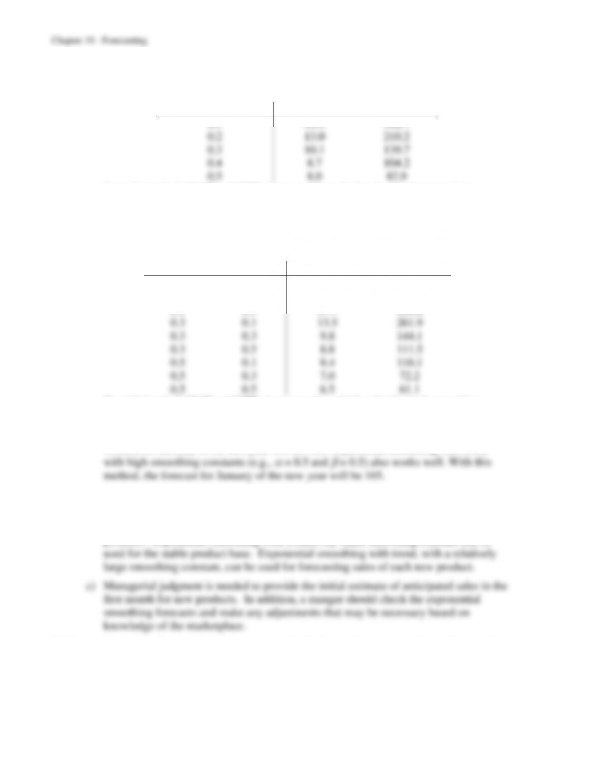
Moving-average method:
3
4
5
6
7
8
9
10
11
12
13
14
15
16
17
18
B C D E F G H
Mo ving
Time True Average Forecastin g Number o f previous
Period Valu e Forecast Error perio ds to consider
1 126 n= 3
2 137 #N/A
3 142 #N/A Mean Absolute Deviation
4 150 135 15 MAD = 8.1
5 153 143 10
6 154 148 6 Mean Sq uare Error
7 148 152 4 MSE = 84.3
8 145 152 7
9 147 149 2
10 151 147 4
11 159 148 11
12 166 152 14
13 159
Comparing MAD values (5.3, 10.0, and 8.1, respectively), the last-value method is the
best to use of these three options.
10–12
c) Using the template for exponential smoothing, with an initial estimate of 120, the
following forecast errors were obtained for various values of the smoothing constant
:
Smoothing Constant
MAD
MSE
0.1
18.5
382.7
0.2
13.0
210.2
0.3
10.1
139.7
0.4
8.7
104.2
0.5
8.0
82.9
Considering both MAD and MSE, it appears that a high value for the smoothing
constant is appropriate.
d) Using the template for exponential smoothing with trend, using initial estimates of 120
for the average value and 10 for the trend, the following forecast errors were obtained
for various values of the smoothing constants
and
:
MAD
MSE
0.1
0.1
25.4
919.6
0.1
0.3
21.2
634.1
0.1
0.5
17.7
450.6
0.3
0.1
13.5
261.9
0.3
0.3
9.8
144.1
0.3
0.5
8.8
111.5
0.5
0.1
8.4
116.1
0.5
0.3
7.0
72.2
0.5
0.5
6.5
61.1
Considering both MAD and MSE, it appears that a high value for both smoothing
constants is appropriate.
e) Management should use the last-value method to forecast sales. Using this method the
forecast for January of the new year will be 166. Exponential smoothing with trend
10.23 a) Shift in total sales may be due to the release of new products on top of a stable product
base, as was seen in the CCW case study.
b) Forecasting might be improved by breaking down total sales into stable and new
products. Exponential smoothing with a relatively small smoothing constant can be
10.24 a) Answers will vary. Last value seems to do the best, with exponential smoothing with
trend a close second.
10–13
b) For last value, a change in April will only affect the May forecast.
For averaging, a change in April will affect all forecasts after April.
c) Answers will vary. last value or exponential smoothing seem to do better than the
10.25 a) Using the template for exponential smoothing, with an initial estimate of 50, the
following MAD values were obtained for various values of the smoothing constant
:
Smoothing
Constant
MAD
0.1
1.49
0.2
1.58
0.3
1.67
0.4
1.76
0.5
1.86
b) Using the template for exponential smoothing, with an initial estimate of 50, the
following MAD values were obtained for various values of the smoothing constant
:
Smoothing
Constant
MAD
0.1
1.69
0.2
1.66
0.3
1.71
0.4
1.82
0.5
1.93
c) Using the template for exponential smoothing, with an initial estimate of 50, the
following MAD values were obtained for various values of the smoothing constant
:
Smoothing
Constant
MAD
0.1
2.18
0.2
1.73
0.3
1.59
0.4
1.49
0.5
1.44
10–14
10.26 a) Using the template for exponential smoothing with trend, with an initial estimates of 50
Smoothing
Constant
MAD
0.1
0.74
0.2
0.75
0.3
0.76
0.4
0.77
0.5
0.78
b) Using the template for exponential smoothing with trend, with an initial estimates of 50
obtained for various values of the smoothing constant
:
Smoothing
Constant
MAD
0.1
2.61
0.2
2.76
0.3
2.87
0.4
2.99
0.5
3.05
c) Using the template for exponential smoothing with trend, with an initial estimates of 50
for the average and 2 for the trend and
= 0.2, the following MAD values were
obtained for various values of the smoothing constant
:
Smoothing
Constant
MAD
0.1
5.66
0.2
6.02
0.3
6.23
0.4
6.36
0.5
6.54
10.27 a) The time series is not stable enough for the moving-average method. There appears to
be an upward trend.
10–15
b) Moving Average (n = 3):
3
4
5
6
7
8
9
10
11
12
13
14
15
16
B C D E F G H
Moving
Time True Average Forecasting Number of previous
Period Value Forecast Error periods to consider
1 382 n= 3
2 405 #N/A
3 398 #N/A Mean Absolu te Deviatio n
4 421 395 26 MAD = 16.6
5 426 408 18
6 415 415 0 Mean Square Error
7 443 421 22 MSE = 346.0
8 451 428 23
9 446 436 10
10 464 447 17
11 454
c) Exponential smoothing:
3
4
5
6
7
8
9
10
11
12
13
14
15
16
B C D E F G H
Expon ential
Time True Smoothing Forecasting
Period Valu e Forecast Error Smoothing Constant
1 382 380 2 = 0.5
2 405 381 24
3 398 393 5 Initial Estimate
4 421 396 26 Average = 380
5 426 408 18
6 415 417 2 Mean Absolute Deviation
7 443 416 27 MAD = 15.14
8 451 430 21
9 446 440 6 Mean Sq u are Error
10 464 443 21 MSE = 322.97
11 454
d) Exponential smoothing with trend:
3
4
5
6
7
8
9
10
11
12
13
14
15
16
17
B C D E F G H I J
Exponential
Time True Latest Estimated Smoothing Forecasting
Period Valu e Trend Tren d Forecast Error Smoothing Constants
1 382 10.00 380 2 = 0.25
2 405 10.50 10.13 391 14 = 0.25
3 398 13.72 11.02 405 7
4 421 9.21 10.57 414 7 Initial Estimates
5 426 12.32 11.01 427 1 Average = 370
6 415 10.82 10.96 438 23 Trend = 10
7 443 5.33 9.55 441 2
8 451 9.94 9.65 451 0 Mean Absolute Deviatio n
9 446 9.53 9.62 461 15 MAD = 7.28
10 464 5.87 8.68 466 2
11 8.20 8.56 474 Mean Square Error
12 #N/A MSE = 105.11
e) Based on the MAD and MSE values, exponential smoothing with trend should be used
in the future.

10–16
10.28 For moving average, the forecast typically lie below the demands.
For exponential smoothing, the forecasts typically lie below the demands.
10.29 Forecast for next production yield = 62%.
3
4
5
6
7
8
9
10
11
12
13
14
15
16
17
B C D E F G H I J
Exponential
Time True Latest Estimated Smooth ing Forecasting
Period Value T rend T rend Forecast Error Smooth ing Constan ts
115 5.00 15 0 = 0.2
221 5.00 5.00 20 1 = 0.2
324 5.20 5.04 25 1
432 4.79 4.99 30 2Initial Estimates
537 5.39 5.07 35 2 Average = 10
641 5.38 5.13 41 0 T rend = 5
740 5.15 5.14 46 6
847 3.93 4.89 50 3Mean Absolute Deviatio n
951 4.35 4.79 54 3 MAD = 2.27
10 53 4.19 4.67 58 5
11 3.66 4.46 62 Mean Sq uare Error
12 #N/A MSE = 8.75
10.30 a) Seasonal factors:
3
4
5
6
7
8
9
10
11
12
13
14
15
16
B C D E F G
True
Year Quarter Value Type of Seasonality
1 1 25 Quarterly
1 2 47
1 3 68
1 4 42 Estimate for
2 1 27 Quarter Seasonal Factor
2 2 46 1 0.550
2 3 72 2 1.027
2 4 39 3 1.519
3 1 24 4 0.904
3 2 49
3 3 70
3 4 44
10–17
b) Last-value method with seasonality forecast = 27 acre-feet.
3
4
5
6
7
8
9
10
11
12
13
14
15
16
17
18
19
20
21
22
23
24
25
26
B C D E F G H I J K
Seasonally Seasonally
T rue Adjusted Adjusted Actu al Fo recastin g
Year Quarter Value Valu e Fo recast Forecast Error Type o f Season ality
1 1 25 45 Quarterly
1 2 47 46 45 47 0
1 3 68 45 46 70 2Quarter Season al F actor
1 4 42 46 45 40 2 1 0.550
2 1 27 49 46 26 1 2 1.027
2 2 46 45 49 50 4 3 1.519
2 3 72 47 45 68 4 4 0.904
2 4 39 43 47 43 41.000
3 1 24 44 43 24 01.000
3 2 49 48 44 45 41.000
3 3 70 46 48 72 21.000
3 4 44 49 46 42 21.000
4 1 #N/A 49 27 1.000
4 2 #N/A #N/A 1.000
4 3 #N/A #N/A 1.000
4 4 #N/A #N/A
5 1 #N/A #N/A Mean Ab solute Deviatio n
5 2 #N/A #N/A MAD = 2.39
5 3 #N/A #N/A
5 4 #N/A #N/A Mean Sq uare Error
6 1 #N/A #N/A MSE = 7.82
c) Winter = (49)(0.550) = 27
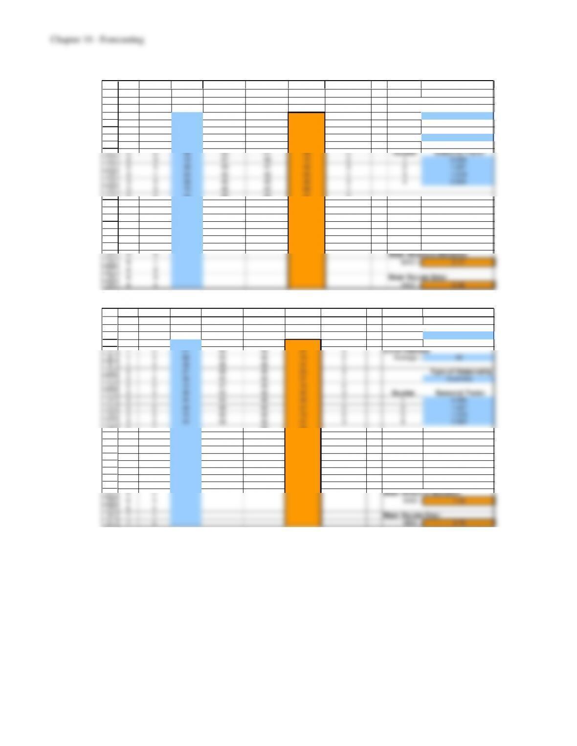
d) Averaging method with seasonality forecast = 25 acre-feet.
3
4
5
6
7
8
9
10
11
12
13
14
15
16
17
18
19
20
21
22
23
24
25
26
B C D E F G H I J K
Seasonally Seasonally
T rue Adjusted Adjusted Actu al Fo recastin g
Year Quarter Value Valu e Fo recast Forecast Error Type o f Season ality
1 1 25 45 Quarterly
1 2 47 46 45 47 0
1 3 68 45 46 69 1Quarter Season al F actor
1 4 42 46 45 41 1 1 0.550
2 1 27 49 46 25 2 2 1.027
2 2 46 45 46 48 2 3 1.519
2 3 72 47 46 70 2 4 0.904
2 4 39 43 46 42 31.000
3 1 24 44 46 25 11.000
3 2 49 48 46 47 21.000
3 3 70 46 46 70 01.000
3 4 44 49 46 41 31.000
4 1 #N/A 46 25 1.000
4 2 #N/A #N/A 1.000
4 3 #N/A #N/A 1.000
4 4 #N/A #N/A
5 1 #N/A #N/A Mean Ab solute Deviatio n
5 2 #N/A #N/A MAD = 1.57
5 3 #N/A #N/A
5 4 #N/A #N/A Mean Sq uare Error
6 1 #N/A #N/A MSE = 3.07
10–18
e) Moving-average method with seasonality forecast = 26 acre-feet.
3
4
5
6
7
8
9
10
11
12
13
14
15
16
17
18
19
20
21
22
23
24
25
26
27
28
29
B C D E F G H I J K
Seasonally Season ally
T rue Adjusted Adjusted Actu al Fo recasting Number of p revious
Year Quarter Valu e Valu e Fo recast Forecast Error periods to con sid er
1 1 25 45 n = 4
1 2 47 46 #N/A
1 3 68 45 #N/A T yp e of Season ality
1 4 42 46 #N/A Q uarterly
2 1 27 49 46 25 2
2 2 46 45 47 48 2Qu arter Season al F actor
2 3 72 47 46 70 2 1 0.550
2 4 39 43 47 42 3 2 1.027
3 1 24 44 46 25 1 3 1.519
3 2 49 48 45 46 3 4 0.904
3 3 70 46 45 69 11.000
3 4 44 49 45 41 31.000
4 1 #N/A 47 26 1.000
4 2 #N/A #N/A 1.000
4 3 #N/A #N/A 1.000
4 4 #N/A #N/A 1.000
5 1 #N/A #N/A 1.000
5 2 #N/A #N/A 1.000
5 3 #N/A #N/A
5 4 #N/A #N/A Mean Absolu te Deviation
6 1 #N/A #N/A MAD = 2.17
6 2 #N/A #N/A
6 3 #N/A #N/A Mean Sq u are Error
6 4 #N/A #N/A MSE = 5.46
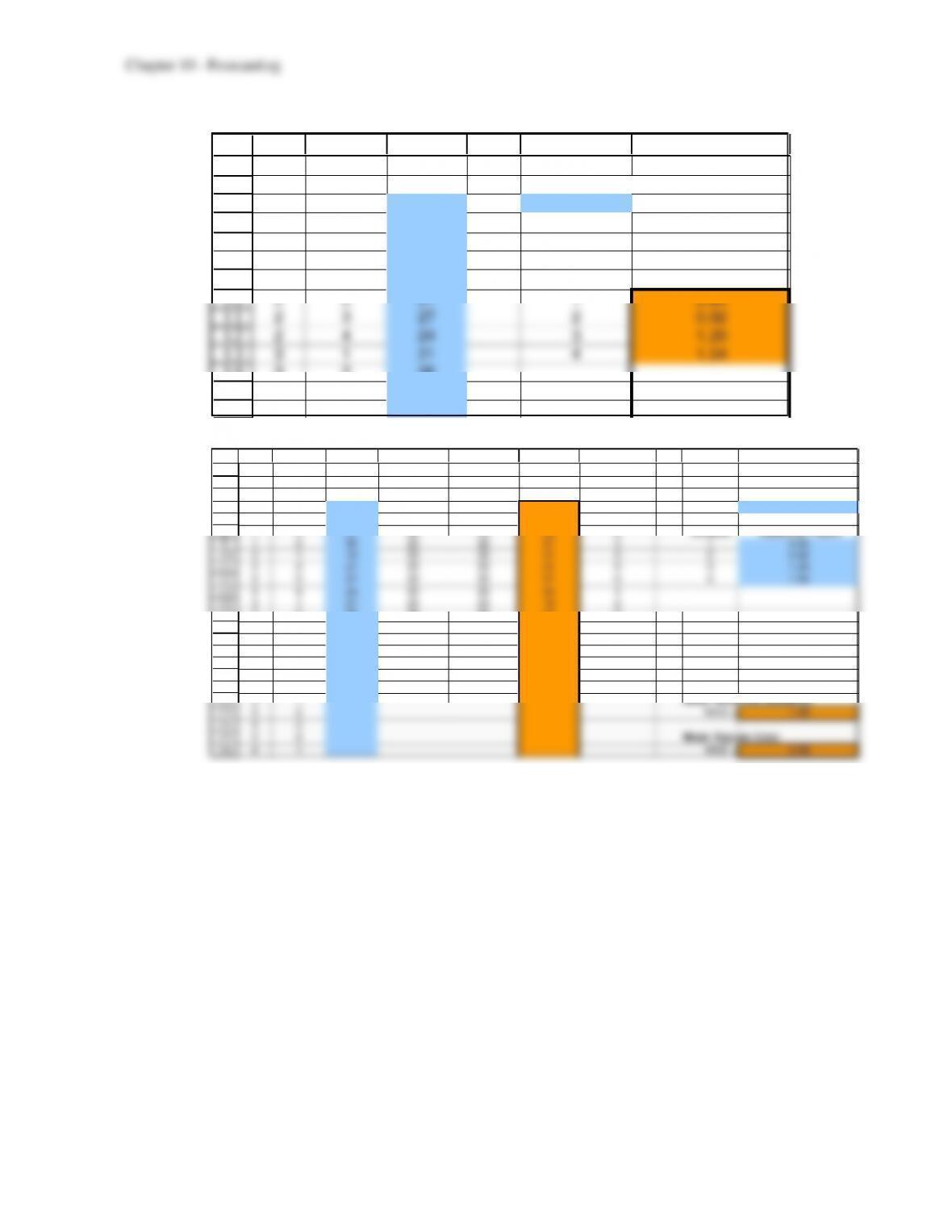
f) Exponential smoothing method with seasonality forecast = 25 acre-feet.
3
4
5
6
7
8
9
10
11
12
13
14
15
16
17
18
19
20
21
22
23
24
25
26
27
28
29
30
31
B C D E F G H I J K
Season ally Seasonally
T rue Adju sted Adjusted Actu al Forecasting Smoothing Constant
Year Qu arter Valu e Value F orecast F orecast Error = 0.1
1 1 25 45 46 25 0
1 2 47 46 46 47 0Initial Estimate
1 3 68 45 46 70 2 Average = 46
1 4 42 46 46 41 1
2 1 27 49 46 25 2Type of Season ality
2 2 46 45 46 47 1 Quarterly
2 3 72 47 46 70 2
2 4 39 43 46 42 3Qu arter Season al Factor
3 1 24 44 46 25 1 1 0.550
3 2 49 48 46 47 2 2 1.027
3 3 70 46 46 70 0 3 1.519
3 4 44 49 46 41 3 4 0.904
4 1 #N/A 46 25 1.000
4 2 #N/A #N/A 1.000
4 3 #N/A #N/A 1.000
4 4 #N/A #N/A 1.000
5 1 #N/A #N/A 1.000
5 2 #N/A #N/A 1.000
5 3 #N/A #N/A 1.000
5 4 #N/A #N/A 1.000
6 1 #N/A #N/A
6 2 #N/A #N/A Mean Absolute Deviatio n
6 3 #N/A #N/A MAD = 1.42
6 4 #N/A #N/A
7 1 #N/A #N/A Mean Square Error
7 2 #N/A #N/A MSE = 2.75
g) The exponential smoothing method results in the lowest MAD value (1.42) and the
lowest MSE value (2.75).
10–19
10.31 a)
3
4
5
6
7
8
9
10
11
12
13
14
15
16
B C D E F G
True
Year Quarter Value Type of Seasonality
1 1 23 Quarterly
1 2 22
1 3 31
1 4 26 Estimate for
2 1 19 Quarter Seasonal Factor
2 2 21 1 0.84
2 3 27 2 0.92
2 4 24 3 1.20
3 1 21 4 1.04
3 2 26
3 3 32
3 4 28
b) Last-value method with seasonality forecast = 23.
3
4
5
6
7
8
9
10
11
12
13
14
15
16
17
18
19
20
21
22
23
24
25
26
B C D E F G H I J K
Seasonally Seasonally
T rue Adjusted Adjusted Actu al Fo recastin g
Year Quarter Value Valu e Fo recast Forecast Error Type o f Season ality
1 1 23 27 Quarterly
1 2 22 24 27 25 3
1 3 31 26 24 29 2Quarter Season al F actor
1 4 26 25 26 27 1 1 0.84
2 1 19 23 25 21 2 2 0.92
2 2 21 23 23 21 0 3 1.20
2 3 27 23 23 27 0 4 1.04
2 4 24 23 23 23 11.000
3 1 21 25 23 19 21.000
3 2 26 28 25 23 31.000
3 3 32 27 28 34 21.000
3 4 28 27 27 28 01.000
4 1 #N/A 27 23 1.000
4 2 #N/A #N/A 1.000
4 3 #N/A #N/A 1.000
4 4 #N/A #N/A
5 1 #N/A #N/A Mean Ab solute Deviatio n
5 2 #N/A #N/A MAD = 1.49
5 3 #N/A #N/A
5 4 #N/A #N/A Mean Sq uare Error
6 1 #N/A #N/A MSE = 3.28
10–20
3
4
5
6
7
8
9
10
11
12
13
14
15
16
17
18
19
20
21
22
23
24
25
26
B C D E F G H I J K
Seasonally Seasonally
T rue Adjusted Adjusted Actu al Fo recastin g
Year Quarter Value Valu e Fo recast Forecast Error Type o f Season ality
1 1 23 27 Quarterly
1 2 22 24 27 25 3
1 3 31 26 26 31 0Quarter Season al F actor
1 4 26 25 26 27 1 1 0.84
2 1 19 23 26 21 2 2 0.92
2 2 21 23 25 23 2 3 1.20
2 3 27 23 25 30 3 4 1.04
2 4 24 23 24 25 11.000
3 1 21 25 24 20 11.000
3 2 26 28 24 22 41.000
3 3 32 27 25 30 21.000
3 4 28 27 25 26 21.000
4 1 #N/A 25 21 1.000
4 2 #N/A #N/A 1.000
4 3 #N/A #N/A 1.000
4 4 #N/A #N/A
5 1 #N/A #N/A Mean Ab solute Deviatio n
5 2 #N/A #N/A MAD = 1.94
5 3 #N/A #N/A
5 4 #N/A #N/A Mean Sq uare Error
6 1 #N/A #N/A MSE = 4.85
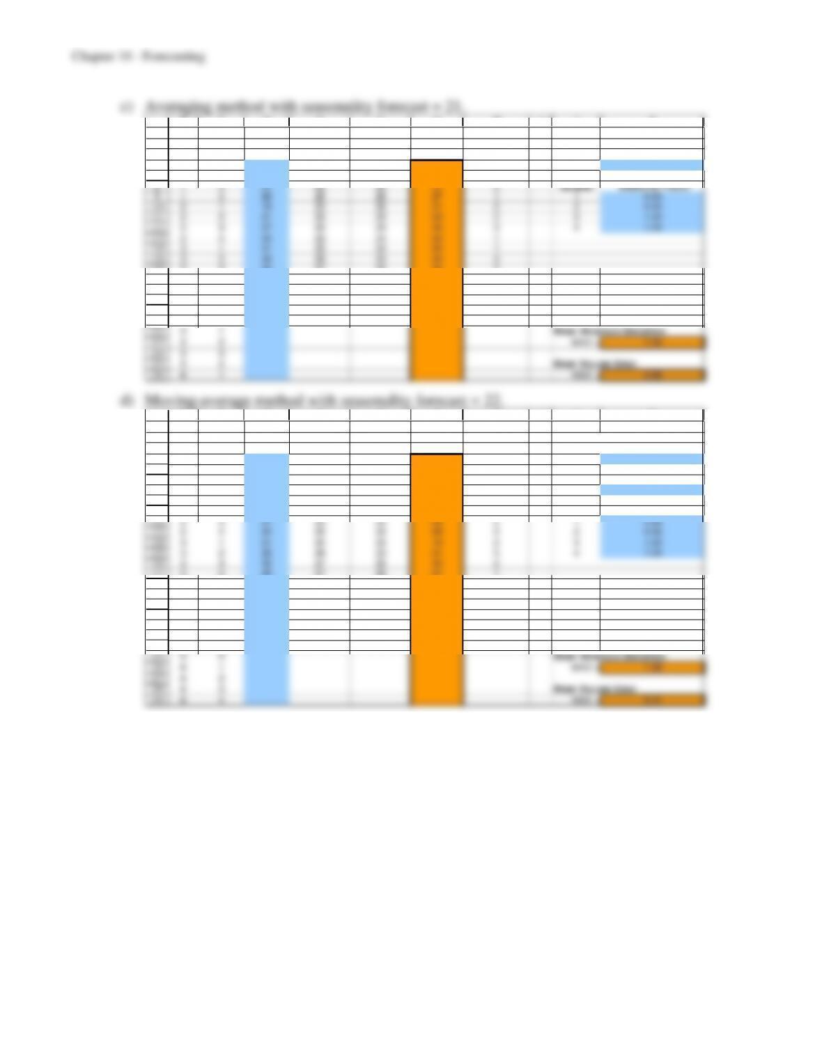
d) Moving-average method with seasonality forecast = 22.
3
4
5
6
7
8
9
10
11
12
13
14
15
16
17
18
19
20
21
22
23
24
25
26
27
28
29
B C D E F G H I J K
Seasonally Season ally
T rue Adjusted Adjusted Actu al Fo recasting Number of p revious
Year Quarter Valu e Valu e Forecast F orecast Error p eriods to consider
1 1 23 27 n = 4
1 2 22 24 #N/A
1 3 31 26 #N/A T yp e of Season ality
1 4 26 25 #N/A Q uarterly
2 1 19 23 26 21 2
2 2 21 23 24 22 1Qu arter Season al F actor
2 3 27 23 24 29 2 1 0.84
2 4 24 23 23 24 0 2 0.92
3 1 21 25 23 19 2 3 1.20
3 2 26 28 23 21 5 4 1.04
3 3 32 27 25 30 21.000
3 4 28 27 26 27 11.000
4 1 #N/A 27 22 1.000
4 2 #N/A #N/A 1.000
4 3 #N/A #N/A 1.000
4 4 #N/A #N/A 1.000
5 1 #N/A #N/A 1.000
5 2 #N/A #N/A 1.000
5 3 #N/A #N/A
5 4 #N/A #N/A Mean Absolu te Deviation
6 1 #N/A #N/A MAD = 1.98
6 2 #N/A #N/A
6 3 #N/A #N/A Mean Sq u are Error
6 4 #N/A #N/A MSE = 5.31