Chapter 06 – Efficient Diversification
CHAPTER 06
6-1
© 2013 by McGraw-Hill Education. This is proprietary material solely for authorized instructor use. Not authorized for sale or
distribution in any manner. This document may not be copied, scanned, duplicated, forwarded, distributed, or posted on a website, in
whole or part.
Chapter 06 – Efficient Diversification
EFFICIENT DIVERSIFICATION
1. So long as the correlation coefficient is below 1.0, the portfolio will benefit from diversification
2. The covariance with the other assets is more important. Diversification is accomplished via
3. a and b will have the same impact of increasing the Sharpe ratio from .40 to .45.
4. The expected return of the portfolio will be impacted if the asset allocation is changed. Since
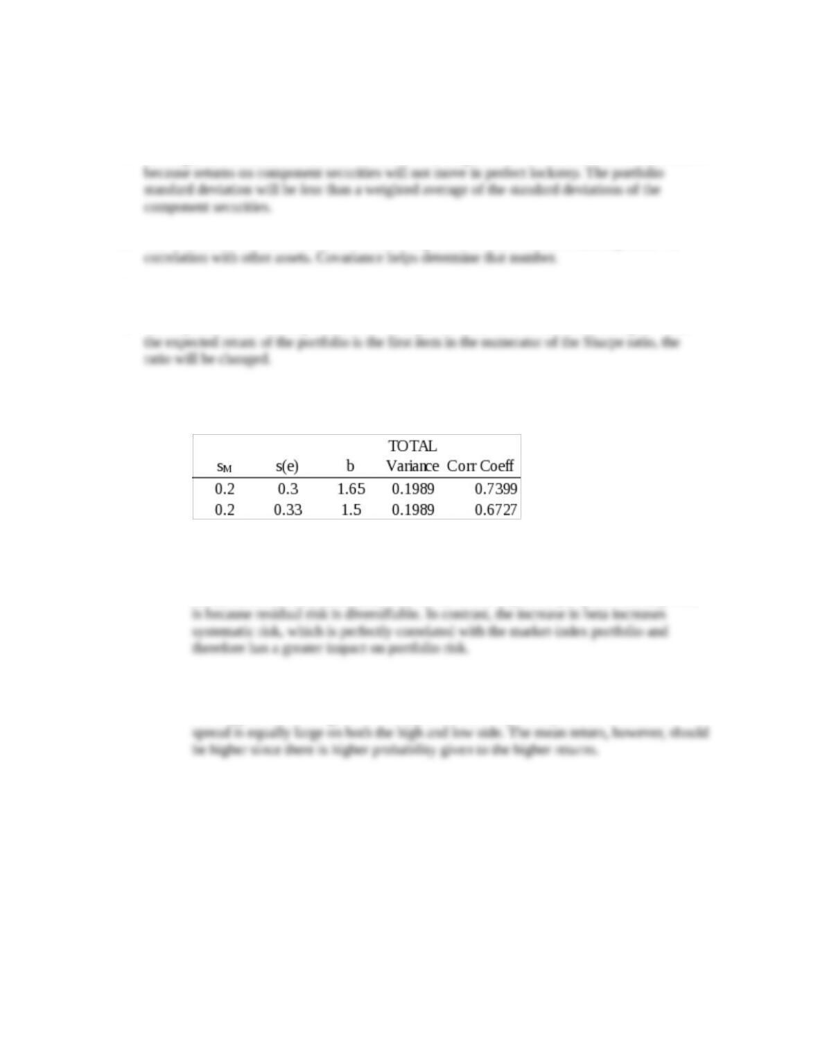
5. Total variance = Systematic variance + Residual variance = β2 Var(rM) + Var(e)
When β = 1.5 and σ(e) = .3, variance = 1.52 × .22 + .32 = .18. In the other scenarios:
a. Both will have the same impact. Total variance will increase from .18 to .1989.
b. Even though the increase in the total variability of the stock is the same in either
scenario, the increase in residual risk will have less impact on portfolio volatility. This
6.
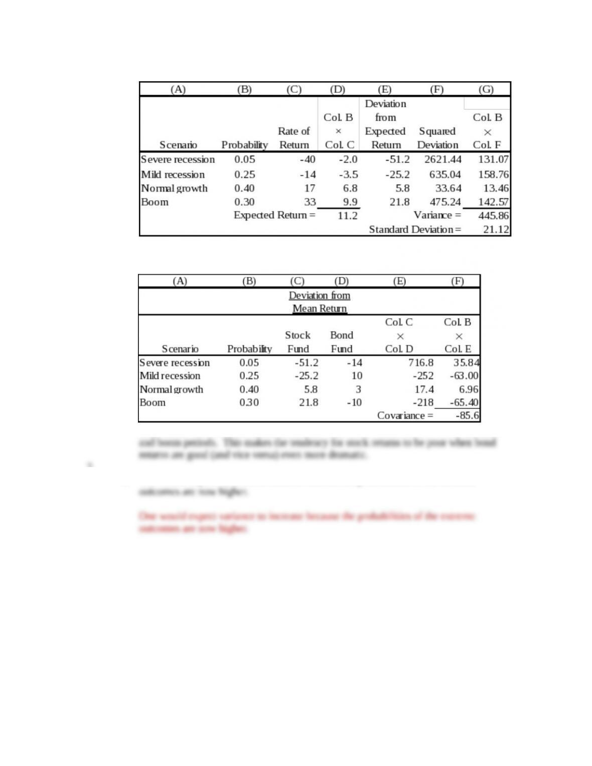
a. Without doing any math, the severe recession is worse and the boom is better. Thus,
there appears to be a higher variance, yet the mean is probably the same since the
6-2
© 2013 by McGraw-Hill Education. This is proprietary material solely for authorized instructor use. Not authorized for sale or
distribution in any manner. This document may not be copied, scanned, duplicated, forwarded, distributed, or posted on a website, in
whole or part.
Chapter 06 – Efficient Diversification
b. Calculation of mean return and variance for the stock fund:
c. Calculation of covariance:
Covariance has increased because the stock returns are more extreme in the recession
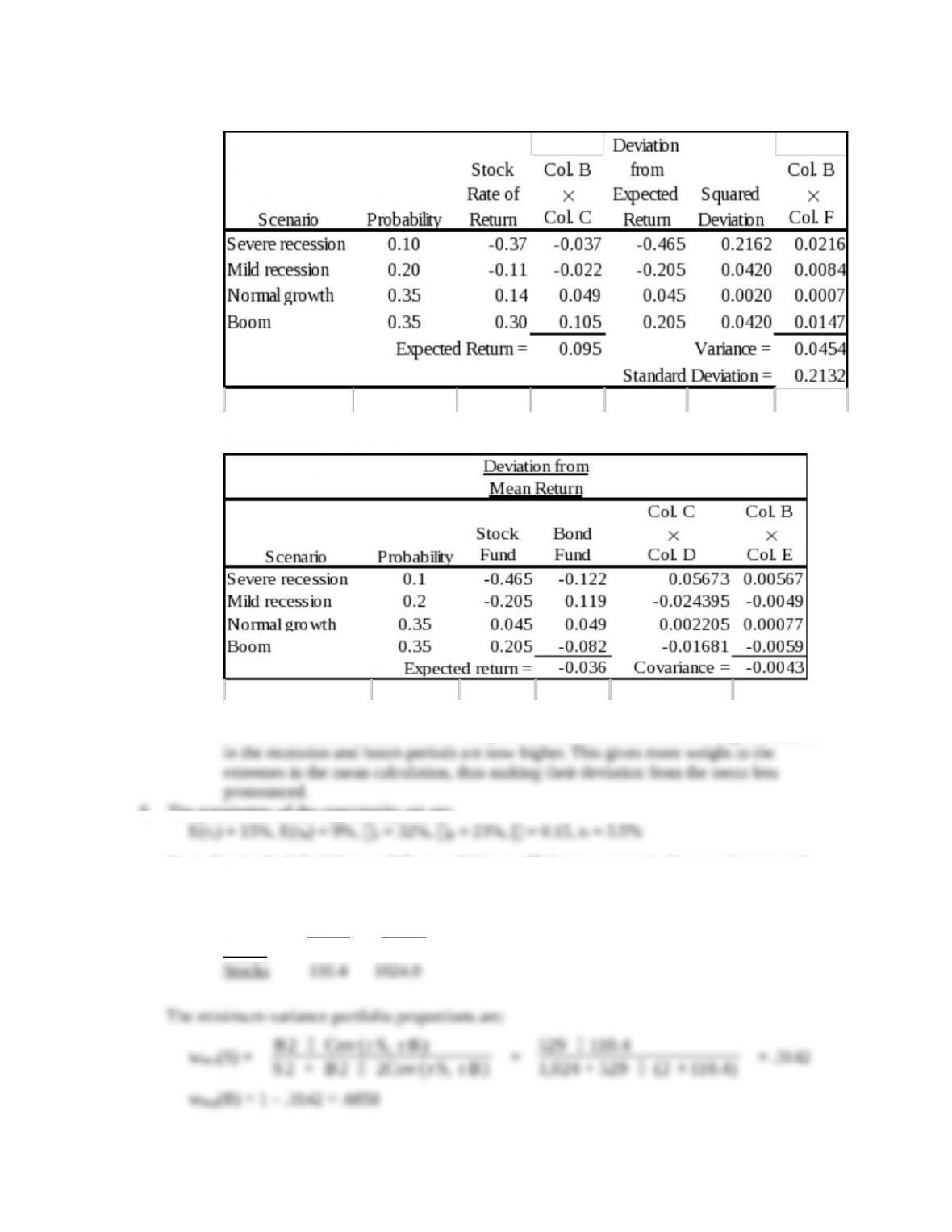
7.
a. One would expect variance to increase because the probabilities of the extreme
6-3
© 2013 by McGraw-Hill Education. This is proprietary material solely for authorized instructor use. Not authorized for sale or
distribution in any manner. This document may not be copied, scanned, duplicated, forwarded, distributed, or posted on a website, in
whole or part.
Chapter 06 – Efficient Diversification
b. Calculation of mean return and variance for the stock fund:
c. Calculation of covariance
Covariance has decreased because the probabilities of the more extreme(ngheo) returns
8. The parameters of the opportunity set are:
From the standard deviations and the correlation coefficient we generate the covariance matrix
[note that Cov(rS, rB) = SB]:
Bonds Stocks
Bonds 529.0 110.4
6-4
© 2013 by McGraw-Hill Education. This is proprietary material solely for authorized instructor use. Not authorized for sale or
distribution in any manner. This document may not be copied, scanned, duplicated, forwarded, distributed, or posted on a website, in
whole or part.
Chapter 06 – Efficient Diversification
15 20 25 30 35 40
0
5
10
15
20
Investment Opportunity Set
St andard Deviat ion (% )
Expect ed Ret urn (% )
9.
6-5
© 2013 by McGraw-Hill Education. This is proprietary material solely for authorized instructor use. Not authorized for sale or
distribution in any manner. This document may not be copied, scanned, duplicated, forwarded, distributed, or posted on a website, in
whole or part.
Chapter 06 – Efficient Diversification
15 20 25 30 35 40
0
5
10
15
20
Investment Opportunity Set
St andard Deviat ion (% )
Expect ed Ret urn (% )
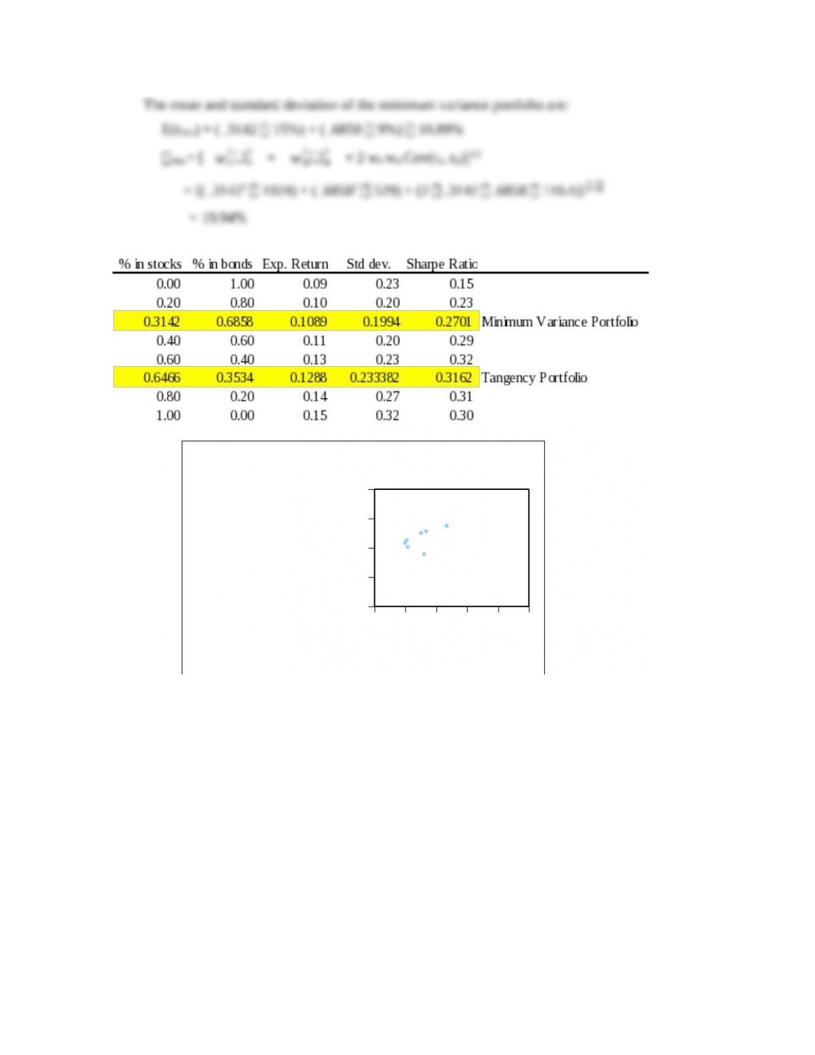
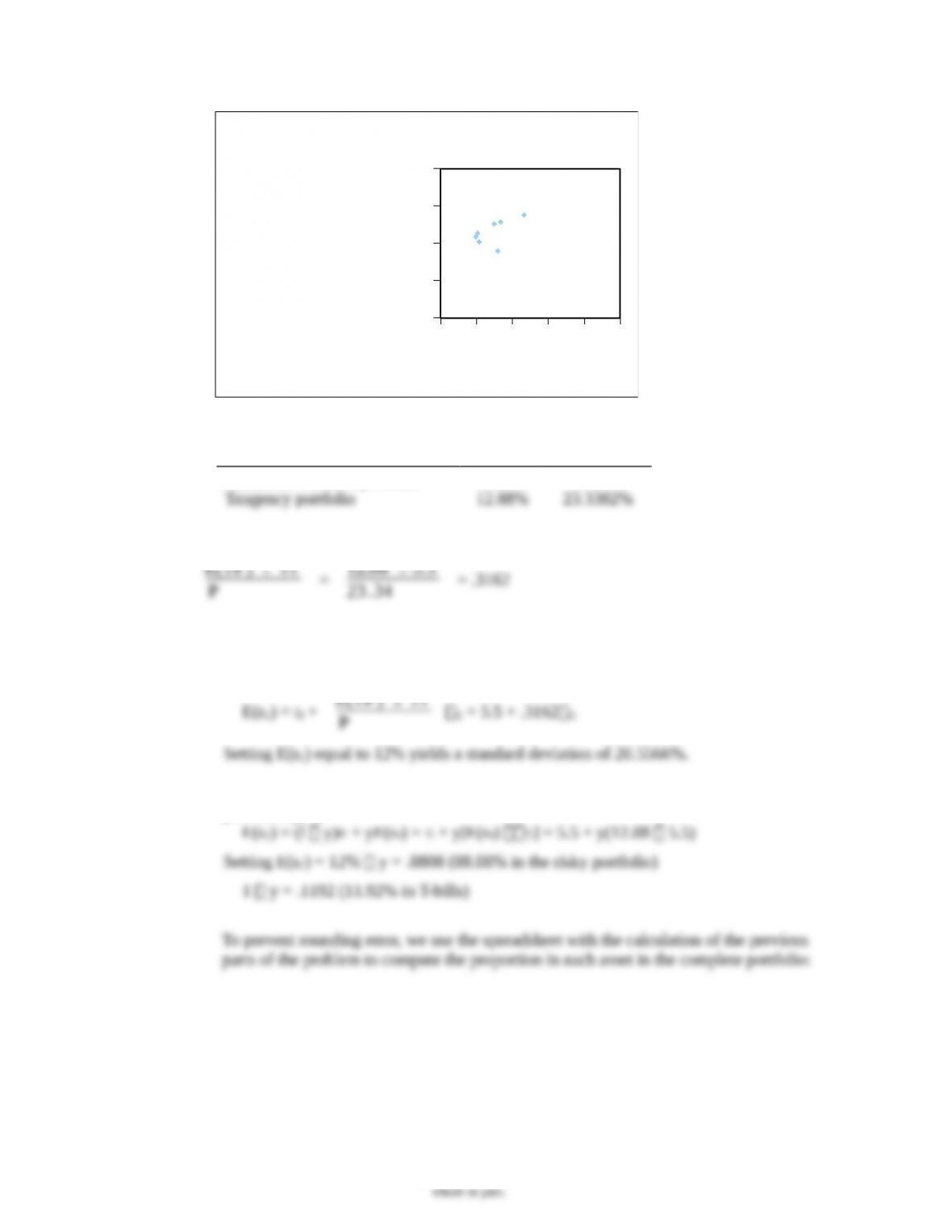
The graph approximates the points:
E(r)
Minimum variance portfolio 10.89% 19.94%
10. The reward-to-variability ratio (Sharpe ratio) of the optimal CAL is:
E( rP ) - r f
P
=
12.88 - 5.5
23 .34
= .3162
11.
a. The equation for the CAL is:
E(rC) = rf +
E( rP ) - r f
P
C = 5.5 + .3162C
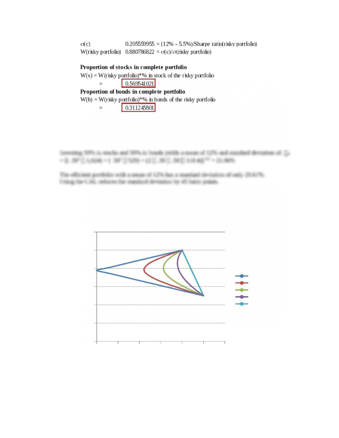
Setting E(rC) equal to 12% yields a standard deviation of 20.5566%.
b. The mean of the complete portfolio as a function of the proportion invested in the risky
portfolio (y) is:
6-6
© 2013 by McGraw-Hill Education. This is proprietary material solely for authorized instructor use. Not authorized for sale or
distribution in any manner. This document may not be copied, scanned, duplicated, forwarded, distributed, or posted on a website, in
whole or part.
Chapter 06 – Efficient Diversification
12. Using only the stock and bond funds to achieve a mean of 12%, we solve:
12 = 15wS + 9(1 wS ) = 9 + 6wS wS = .5
13.
a. Although it appears that gold is dominated by stocks, gold can still be an attractive
diversification asset. If the correlation between gold and stocks is sufficiently low, gold
will be held as a component in the optimal portfolio.
0% 5% 10% 15% 20% 25% 30%
0%
2%
4%
6%
8%
10%
12%
0.05
0.1
Corr = -1
Corr = -0.5
Corr = 0
Corr = 0.5
Corr = 1
b. If gold had a perfectly positive correlation with stocks, gold would not be a part of
efficient portfolios. The set of risk/return combinations of stocks and gold would plot as
a straight line with a negative slope. (Refer to the above graph when correlation is 1.)
The graph shows that when the correlation coefficient is 1, holding gold provides no
6-7
© 2013 by McGraw-Hill Education. This is proprietary material solely for authorized instructor use. Not authorized for sale or
distribution in any manner. This document may not be copied, scanned, duplicated, forwarded, distributed, or posted on a website, in
whole or part.
Chapter 06 – Efficient Diversification
14. Since Stock A and Stock B are perfectly negatively correlated, a risk-free portfolio can be
created and the rate of return for this portfolio in equilibrium will always be the risk-free rate.
To find the proportions of this portfolio [with wA invested in Stock A and wB = (1 –wA )
invested in Stock B], set the standard deviation equal to zero. With perfect negative correlation,
the portfolio standard deviation reduces to:
15. Since these are annual rates and the risk-free rate was quite variable during the sample period of
the recent 20 years, the analysis has to be conducted with continuously compounded rates in
6-8
© 2013 by McGraw-Hill Education. This is proprietary material solely for authorized instructor use. Not authorized for sale or
distribution in any manner. This document may not be copied, scanned, duplicated, forwarded, distributed, or posted on a website, in
whole or part.