Gross margin rate
21.0%
24.0%
(Gross margin/sales)
Inventory turnover
3.1
3.9
(COGS/average inventory)
E9–13. Identifying effects of a LIFO liquidation (LO 5)
LIFO gross margin
Gross margin percentage
Sales revenues, 275 @ $1,350
Cost of goods sold:
275
LIFO gross margin
Gross margin percentage
9-17
Copyright © 2015 McGraw-Hill Education. All rights reserved. No reproduction or distribution without the prior written consent of
McGraw-Hill Education.
percentage is .50. But with the LIFO liquidation, the reported
margin percentage is .529. This mismatch can be avoided by
purchasing enough inventory in any given year to avoid liquidating
old LIFO layers.
E9-14. Eliminating FIFO holding gains (LO 1, 12)
(1) Reported cost of goods sold—FIFO
$ 23,800,000
(2) Beginning Inventory
$ 5,950,000
(3) Rate of increase in purchase costs
0.07
(4) Cost of goods sold @ current costs
= (1) + ((2) x (3))
24,216,500
Realized holding gain in 2014
= (4) – (1)
$ 416,500
E9-15. Correcting inventory errors (LO 1)
(CMA adapted)
The easiest way for students to visualize inventory error adjustment
is to use the cost of goods sold formula and analyze the errors one
at a time. Starting with the 2012 error and assuming beginning 2012
inventory was correctly stated:
2012 Error
Beginning inventory None
$23,000
Since cost of goods sold is understated due to the ending inventory
9-18
must be made to 2013 income—one for the feed-forward effect of
the 2012 error and another for the $61,000 2013 understatement.
2012 Error 2013 Error
overstated by
$23,000
Plus: Purchases None None
Equals: Goods available
overstated by
$23,000
None
Minus: Ending inventory None
understated by
$61,000
overstated by
$23,000
$61,000
Therefore, 2013 cost of goods sold is overstated by $84,000, and
income is understated by this amount. The corrected 2013 income
is $254,000 + $84,000 = $338,000.
The 2014 computation is:
2013 Error 2014 Error
Beginning inventory
understated by
$61,000
None
Plus: Purchases None None
understated by
$61,000
9-19
E9-16. Applying lower of cost or market (LO 10)
(AICPA adapted)
Moore should use the historical cost of $45 in pricing product #2
ending inventory. The rule is the lower of cost or market. The
E9-17. Computing dollar-value LIFO (LO 13)
(AICPA adapted)
To compute ending inventory at base year prices, we need to divide
the year-end prices of each year by the respective price index, then
separate the layers to compute ending inventory at LIFO Cost. Here
are the computations:
Year Ended
December 31,
Inventory at
Respective
Year-End Prices
External
Price Index
(Base Year 2002)
Inventory at
Base Year
(2002) Price
2012
$363,000
1.10
$330,000
2013
$420,000
1.20
$350,000
2014
$430,000
1.25
$344,000
December 31, 2012
9-20
E9-18. Computing dollar-value LIFO (LO 13)
(AICPA adapted)
The computation of dollar value LIFO can be seen below. The first
step is to find the base-year price of ending inventory. We can do
Ending inventory
Price
Index
Base-Year Price
$780,000
1.2
$650,000
Layers at Base-Year Price
Price
Index
Ending Inventory
at LIFO Cost
$600,000
1.0
$600,000
_$50,000
1.2
__60,000
$650,000
$660,000
E9–19. Evaluating inventory costing concepts (LO 5, 9, 10)
(AICPA adapted)
Requirement 1:
Description of fundamental cost flow assumption:
a) It is difficult, if not impossible, to measure the physical flow of
goods and, therefore, to cost items on an average price basis
9-21
Requirement 2:
Reasons for using LIFO in an inflationary environment:
In an inflationary economy, LIFO is a useful tool. When using LIFO,
Requirement 3:
Proper accounting treatment when utility of goods is below cost:
The prevailing accounting treatment in this case is to value the
inventory at the lower of cost or market. Lower of cost or market can
9-22
Financial Reporting and Analysis (5th Ed.)
Chapter 9 Solutions
Inventories
Problems/Discussion Questions
Problems
P9–1. Calculating amounts and ratios under FIFO and LIFO (LO 2, 5)
Requirement 1:
Units
Total purchases—2013
550
Total sales—2013
(440)
Ending inventory—2013
110
Beginning inventory—2014
110
Total purchases—2014
530
Goods available for sale—2014
640
Total sales—2014
(510)
Ending inventory—2014
130
Ending inventory 2013—FIFO:
Units
Cost/unit
Total
December 5, 2013
50
$ 32
$ 1,600
September 3, 2013
60
31
1,860
Ending inventory 2013—FIFO
110
$ 3,460
Cost of goods sold 2013—FIFO:
Total purchases—2013
$15,820
Ending inventory 2013—FIFO
(3,460)
Cost of goods sold 2013—FIFO
$12,360
Total sales—2013
$22,925
Cost of goods sold 2013—FIFO
(12,360)
Gross margin—2013
$10,565
9-23
Ending inventory 2014—FIFO:
Units
Cost/unit
Total
November 3, 2014
80
$ 27
$ 2,160
August 20, 2014
50
28
1,400
Ending inventory 2014—FIFO
130
$ 3,560
Cost of goods sold 2014—FIFO:
Beginning inventory 2014—FIFO
$ 3,460
Total purchases—2014
15,510
Ending inventory 2014—FIFO
(3,560)
Cost of goods sold 2014—FIFO
$15,410
Total sales—2014
$26,200
Cost of goods sold 2014—FIFO
(15,410)
Gross margin—2014
$10,790
Requirement 2:
Ending inventory 2013—LIFO:
Units
Cost/unit
Total
January 1, 2013
85
$ 25
$ 2,125
March 15, 2013
25
27
675
Ending inventory 2013—LIFO
110
$ 2,800
Cost of goods sold 2013—LIFO:
Total purchases—2013
$15,820
Ending inventory 2013—LIFO
(2,800)
Cost of goods sold 2013—LIFO
13,020
Total sales—2013
$22,925
Cost of goods sold 2013—LIFO
(13,020)
Gross margin—2013
$ 9,905
Ending inventory 2014—LIFO:
Units
Cost/unit
Total
January 1, 2013
85
$ 25
$ 2,125
March 15, 2013
25
27
675
February 20, 2014
20
31
620
Ending inventory 2014—LIFO
130
$ 3,420
Cost of goods sold 2014—LIFO:
9-24
Beginning inventory 2014—LIFO
$ 2,800
Total purchases—2014
15,510
Ending inventory 2014—LIFO
(3,420)
Cost of goods sold 2014—LIFO
$14,890
Total sales—2014
$26,200
Cost of goods sold 2014—LIFO
(14,890)
Gross margin—2014
$11,310
P9–2. Determining income statement amounts for a manufacturer (LO
1,3, 4)
Requirement 1:
Computation of cost of raw materials used:
Cost of raw materials used = Beginning balance in raw material
= $126,000 + $112,000 + $55,000 + $25,000 + $10,000 + $5,000
– $145,000 = $188,000
Requirement 3:
P9–3. Determining cost of sales under different flow assumptions —
comprehensive (LO 2, 5, 6)
Requirement 1:
9-26
Weighted
Average
Unit cost:
$328,125/60,000 = 5.46875
20,000 x $5.46875 = $109,375
$328,125 − $109,375 = $218,750
LIFO
8,000 x $5.00 = $40,000
$328,125 − $101,600 = $226,525
10,000 x $5.10 = $51,000
2,000 x $5.30 = $10,600
$101,600
equals replacement cost. If the inventory turns quickly, then
inventory replacement cost approximates FIFO inventory. But the
9-27
c) Pros and cons of the accountant’s suggestions.
Pros:
Under periodic LIFO, COGS is computed at 12/31/11, i.e., year-end.
Therefore, the 10,000 units acquired on 12/31/11 would be included
in the COGS for the year 2014. This increases the COGS for the
year and reduces the net income which results in a tax savings.
COGS with the 10,000 units: (10,000 x $6.10) + (6,500 x $6.10)
+ (7,500 x $5.85) + (6,000 x $5.75) + (10,000 x $5.55)
= $234,525
Increase in COGS = $234,525 – $226,525 = $8,000
Tax savings = $8,000 x 0.40 = $3,200.
Cons:
Inventory carrying cost is higher, and the company is exposed to the
risk of an unexpected fall in demand.
Requirement 3 a:
This will be the same as the periodic FIFO method.
Proof:
Cost of Goods Sold under Perpetual FIFO
Date of Sale Units Cost/Unit Total Cost
March 3 _6,000 $5.00 $30,000
9-28
same under FIFO cost flow assumption. However, the answers will
typically be different under LIFO. Under FIFO, the units purchased
on January 1 will be assigned to cost of goods sold first, irrespective
of when cost of goods sold is calculated. On the other hand,
29 will be the first assigned to the cost of goods sold. Under
perpetual LIFO, the cost of goods sold is calculated every time a
new sale is made. On the other hand, the cost of goods sold under
periodic LIFO is calculated only once at the end of the accounting
period. Consequently, they usually result in different values under
perpetual and periodic procedures.
Requirement 3 b:
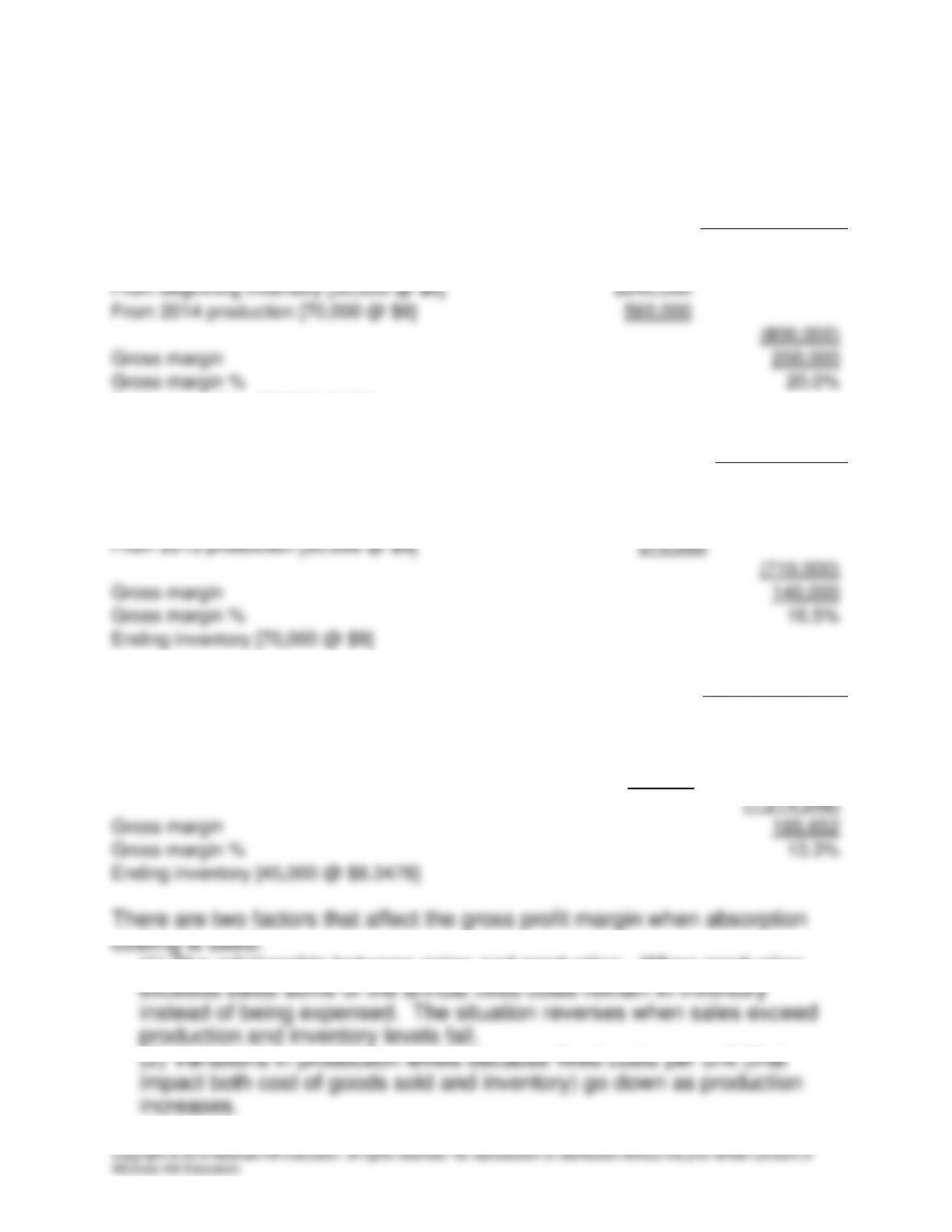
Quantity
Unit cost
1/1 Purchase
8,000
$5.00
$40,000
3/3 Sale
6,000
$5.00
$30,000
Inventory @3/3
2,000
$5.00
$10,000
3/10 Purchase
10,000
$5.10
$51,000
4/15 Purchase
12,000
$5.30
$63,600
24,000
$5.191667
$124,600
9/2 Sale
24,000
$5.191667
$124,600
0
0
9/11 Purchase
10,000
$5.55
$55,500
11/12 Purchase
6,000
$5.75
$34,500
12/1 Purchase
7,500
$5.85
$43,875
Inventory @12/5
23,500
$5.696809
$133,875
12/5 Sale
10,000
$5.696809
$56,968
Inventory @12/5
13,500
$5.696809
$76,907
12/29 Purchase
6,500
$6.10
$39,650
12/31 Inventory
20,000
$5.827846
$116,557
Cost of goods sold under perpetual weighted average = $30,000 +
$124,600 + $56,968 = $211,568. Ending inventory + cost of goods
sold = goods available for sale = $211,568 + $116,557 = $328,125.
9-29
P9-4. Determining the effects of absorption and variable costing
(LO 4)
Requirement 1:
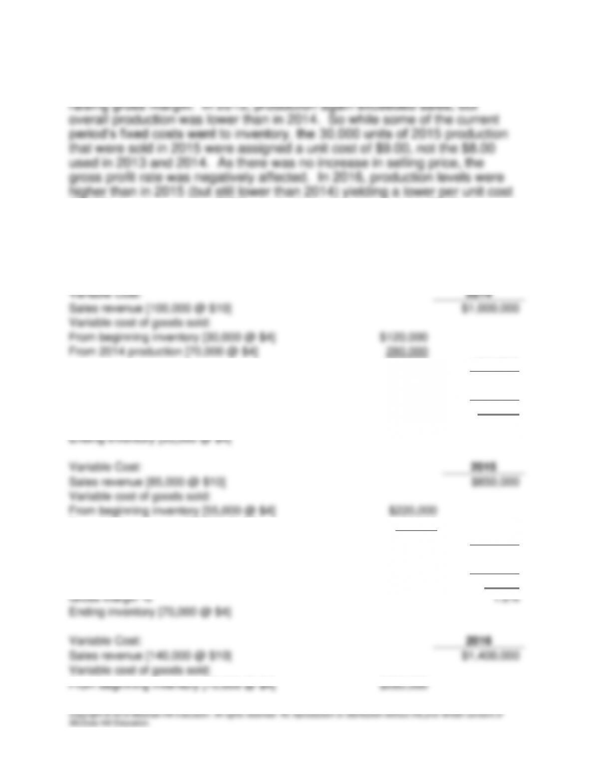
Absorption Cost:
2014
Sales revenue [100,000 @ $10]
$1,000,000
Cost of goods sold:
From beginning inventory [30,000 @ $8]
$240,000
From 2014 production [70,000 @ $8]
560,000
(800,000)
Gross margin
200,000
Gross margin %
20.0%
Ending inventory [55,000 @ $8]
Absorption Cost:
2015
Sales revenue [85,000 @ $10]
$850,000
Cost of goods sold:
From beginning inventory [55,000 @ $8]
$440,000
From 2015 production [30,000 @ $9]
270,000
(710,000)
Gross margin
140,000
Gross margin %
16.5%
Ending inventory [70,000 @ $9]
Absorption Cost:
2016
Sales revenue [140,000 @ $10]
$1,400,000
Cost of goods sold:
From beginning inventory [70,000 @ $9]
$630,000
From 2016 production [70,000 @ $8.3478]
584,348
(1,214,348)
Gross margin
185,652
Gross margin %
13.3%
Ending inventory [45,000 @ $8.3478]
(1) The relationship between sales and production. When production
9-30
Considering these factors in regards to Mastrolia’s data we find that in 2014,
production exceeded sales (as was the case in the previous year) thus
($8.35); however, under FIFO, much of the inventory sold in 2016 was
deemed to be 2015 production which carries a $9.00/unit cost.
Furthermore, none of the 2016 sales carried an $8.00/unit cost as in 2014.
Thus, 2016 gross profit continued its downward trend.
Requirement 2:
Variable Cost:
2014
Sales revenue [100,000 @ $10]
$1,000,000
Variable cost of goods sold:
From beginning inventory [30,000 @ $4]
$120,000
From 2014 production [70,000 @ $4]
280,000
(400,000)
Variable contribution margin
600,000
Less: Fixed production costs
(500,000)
Variable cost gross margin
100,000
Gross margin %
10.0%
Ending inventory [55,000 @ $4]
Variable Cost:
2015
Sales revenue [85,000 @ $10]
$850,000
Variable cost of goods sold:
From beginning inventory [55,000 @ $4]
$220,000
From 2015 production [30,000 @ $4]
120,000
(340,000)
Variable contribution margin
510,000
Less: Fixed production costs
(500,000)
Variable cost gross margin
10,000
Gross margin %
1.2%
Ending inventory [70,000 @ $4]
Variable Cost:
2016
Sales revenue [140,000 @ $10]
$1,400,000
Variable cost of goods sold:
From beginning inventory [70,000 @ $4]
$280,000