9-1
Financial Reporting and Analysis (6th Ed.)
Chapter 9 Solutions
Inventories
Exercises
Exercises
E9–1. Computing inventory amount from income statement data
(LO 1)
(AICPA adapted)
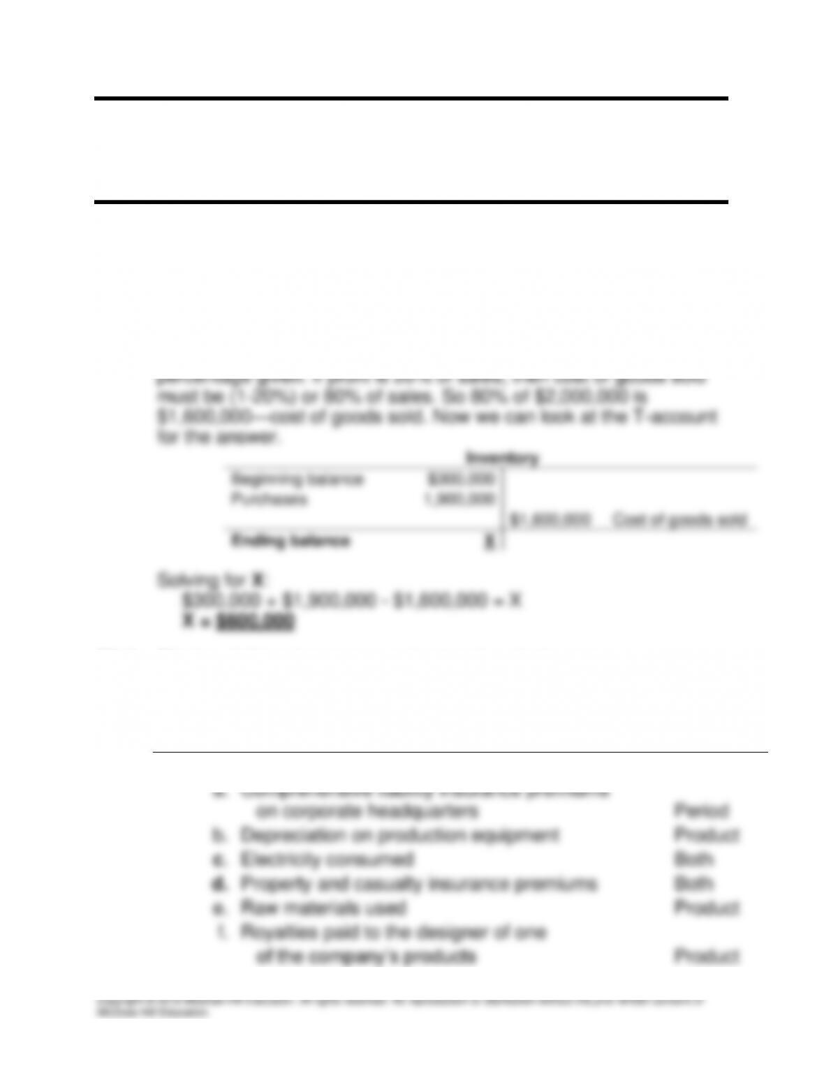
To find merchandise inventory, we first need to find cost of goods
sold. This figure can be computed by using the gross margin
E9–2. Distinguishing between product and period costs
Cost
Nature of incurred cost
Classification
a.
Comprehensive liability insurance premiums
on corporate headquarters
Period
b.
Depreciation on production equipment
Product
c.
Electricity consumed
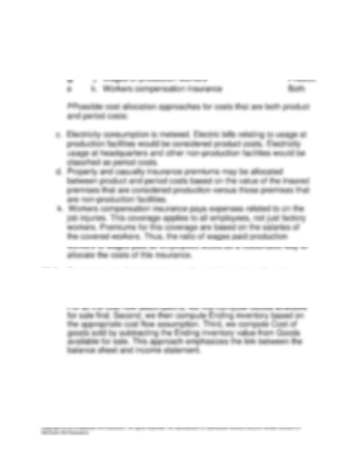
Both
d.
Property and casualty insurance premiums
Both
e.
Raw materials used
Product
f.
Royalties paid to the designer of one
of the company’s products
Product
9-2
N
o
w
Workers compensation insurance
Both
E9–3. Computing ending inventory and cost of goods sold under
different cost flow assumptions (LO 2, 5)
(AICPA adapted)
g.
Salary of corporate legal counsel
Period
h.
Travel expenses for sales force
Period
i.
Wages of plant maintenance personnel
Product
j.
Wages of production workers
Product
9-3
Goods available for sale:
Beginning inventory
300
@ $16
$4,800
Purchase January 14
150
@ $17
2,550
Purchase January 29
100
@ $18
1,800
Units available
550
$9,150
Requirement 1: FIFO
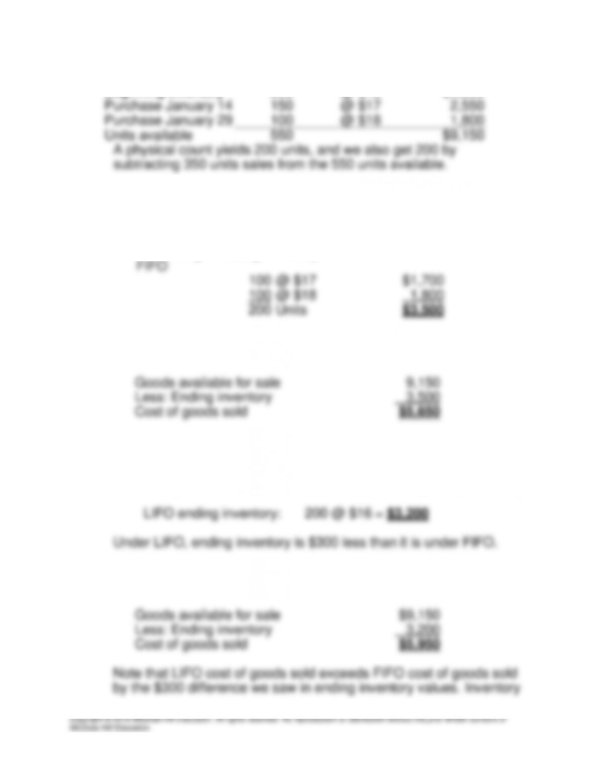
Under FIFO, the most recent purchases are in ending inventory.
Remaining in ending inventory:
FIFO
100
@ $17
$1,700
100
@ $18
1,800
200
Units
$3,500
By subtracting the ending inventory amount of $3,500 from the
goods available for sale, we compute cost of goods sold as follows:
Requirement 2: LIFO
Under LIFO the earliest purchases are assumed to be in ending
inventory. In this case, all the units come from beginning inventory
We compute cost of goods sold the same way we computed it
under FIFO. However, now we subtract LIFO ending inventory.
9-4
is lower, and consequently, Retained earnings and net income are
lower.
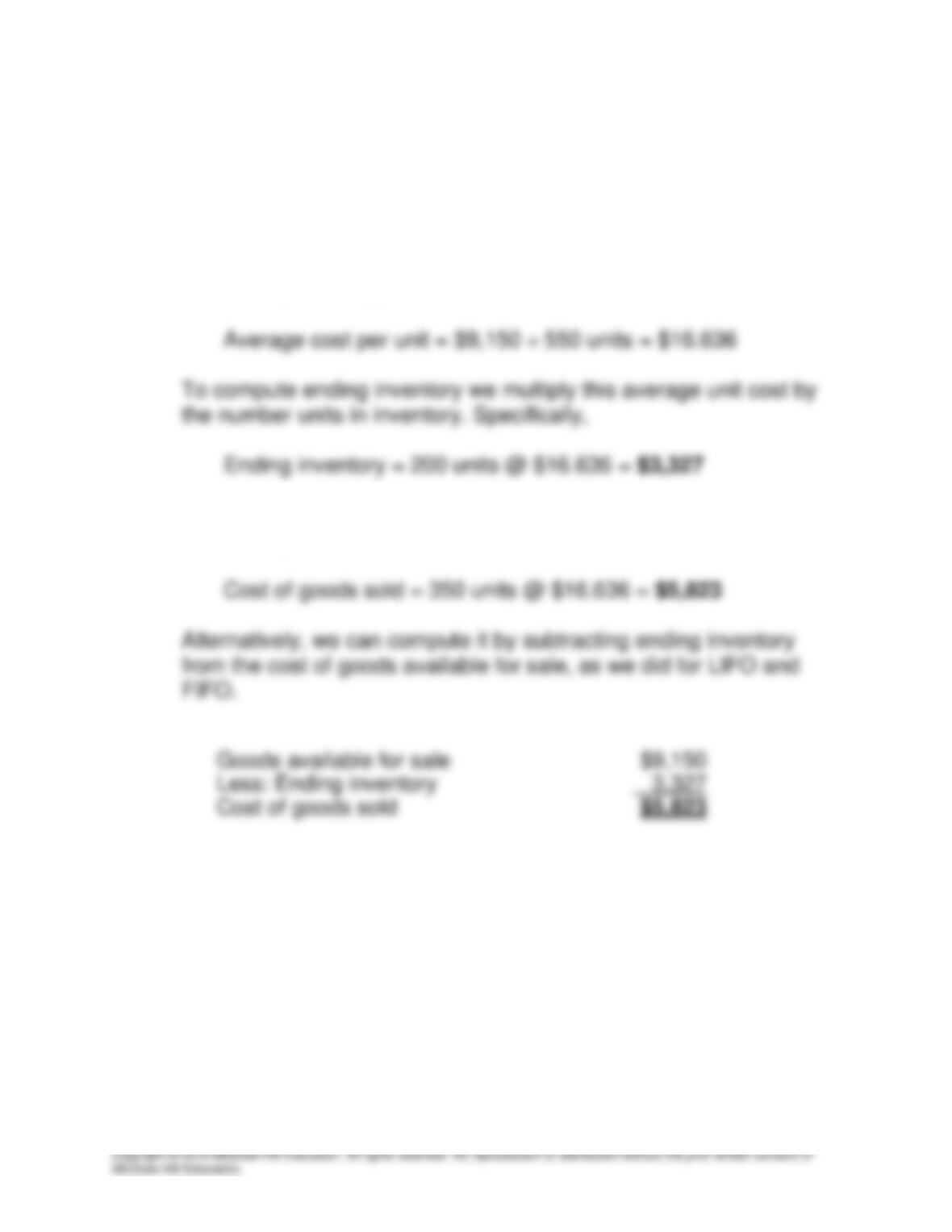
Requirement 3: Average cost
For average cost, we divide goods available for sale by the units
available for sale. These totals come from the first table in our
solution. Specifically,
To compute cost of goods sold, we can multiply the units sold by
this average unit cost as follows:
9-5
E9–4. Computing cost of goods sold (LO 1)
(AICPA adapted)
We can find cost of goods sold for 2014 by analyzing the inventory
account.
Inventory
Beginning balance
$X
Purchases
(Cash + increase in
accounts payable)
$315,000
?
Solve for: Cost of goods sold
Ending balance
$X – 10,000
Purchases can be found by adding together the disbursements for
purchases of merchandise ($290,000) and the increase in trade
accounts payable ($25,000).
We know that the ending balance in inventory is $10,000 less than
the beginning balance. If we began with $X, and purchased
$315,000, and ended with $X – 10,000, we must have sold all
$315,000 that was purchased plus $10,000 of beginning inventory.
Cost of goods sold is $325,000—total purchases plus the decrease
in merchandise inventory.
E9–5. Computing sales from inventory information (LO 3, 4)
(AICPA adapted)
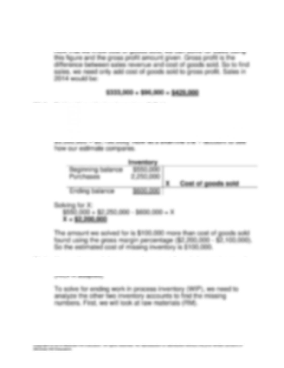
To find Dumas’ sales for 2014, we need to first look at the inventory
T-account.
9-6
X = $333,000
E9–6. Estimating missing inventory (LO 1)
(AICPA adapted)
In this problem, we need to determine the accuracy of the inventory
account. We know that cost of goods sold is 70% of sales [70% of
E9–7. Computing work-in-process inventory from balance sheet and
income statement information (LO 1, 4)
9-7
Raw Materials
Beginning RM
$41,000
Purchases
150,000
X
RM transferred to WIP
(direct materials)
Ending RM
$87,000
We can now solve for X (direct materials).
$41,000 + $150,000 – $87,000 = X
X = $104,000
Now we have direct materials of $104,000 to plug into WIP. But we
also need to know cost of goods manufactured, so we must analyze
finished goods (FG).
Finished Goods
Beginning FG
$173,000
Cost of goods
Manufactured
X
$291,600
Cost of goods sold
Ending FG
$151,000
(Cost of goods sold is 72% of sales of $405,000 or $291,600.)
Once again we can solve for X:
$173,000 + X – $291,600 = $151,000
X = $269,600
Now that we have direct materials and cost of goods manufactured,
we can solve for the ending balance of WIP inventory.
Beginning WIP
$128,000
Direct materials
104,000
Direct labor
112,000
Manufacturing
Overhead
56,000
$269,600
Cost of goods manufactured
Ending WIP
X
9-8
E9–8. Computing inventory under three flow assumptions (LO 2, 5)
(AICPA adapted)
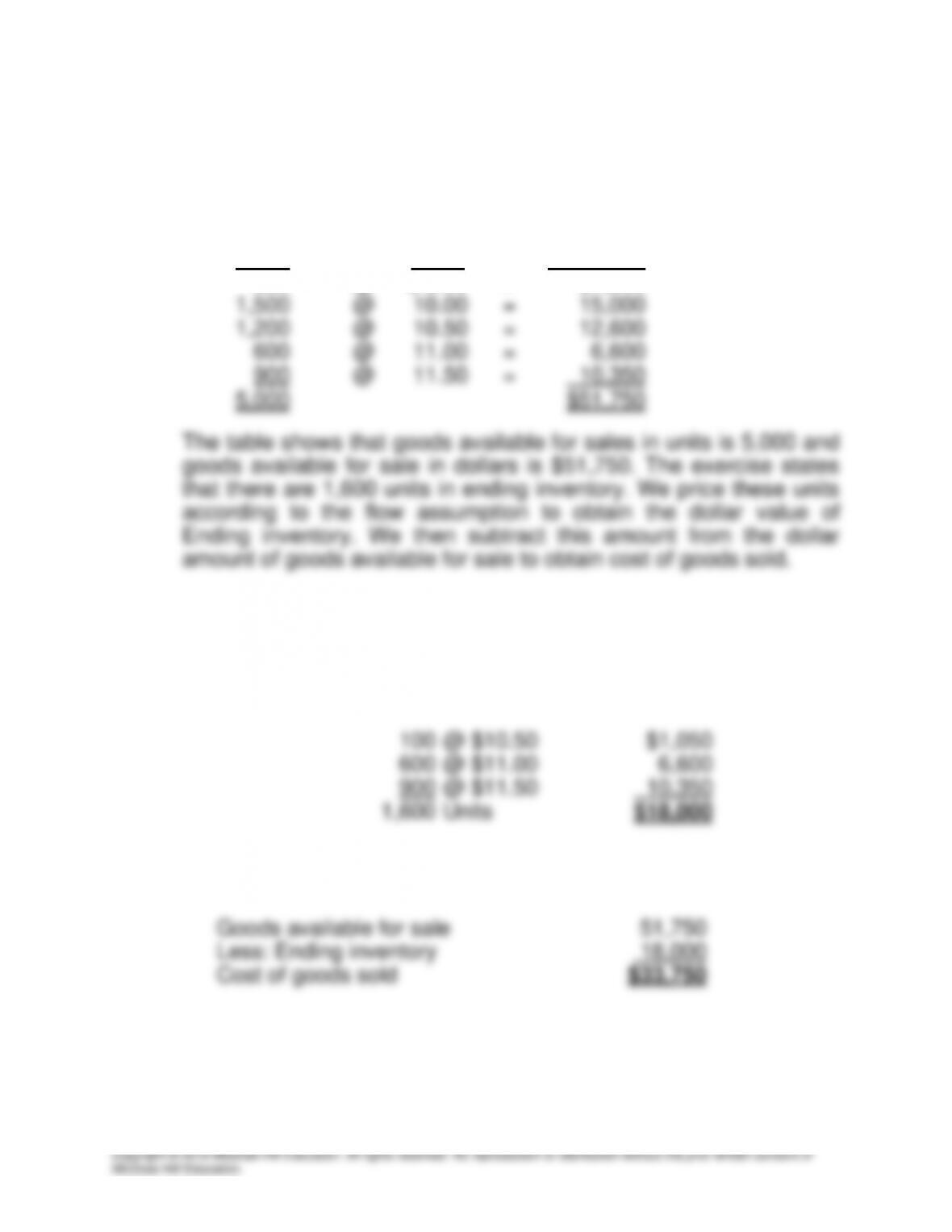
Units and prices for 2014 beginning inventory and purchases are:
Units Price Extended
800 @ $ 9.00 = $7,200
Requirement 1: FIFO
Under FIFO, the most recent purchases are in ending inventory.
Remaining in ending inventory:
100
@ $10.50
$1,050
600
@ $11.00
6,600
900
@ $11.50
10,350
1,600
Units
$18,000
By subtracting the ending inventory amount of $18,000 from the
goods available for sale, we compute cost of goods sold as follows:
9-9
Requirement 2: LIFO
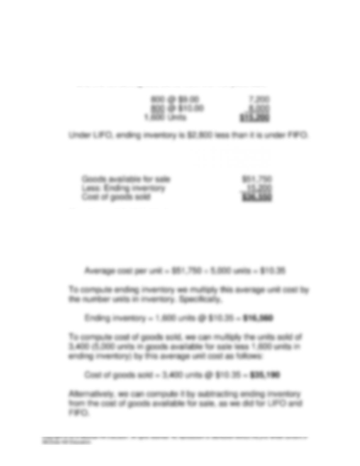
Under LIFO the earliest purchases are assumed to be in ending
inventory. In this case, 800 units come from beginning inventory
and the remaining 800 come from the first purchase.
We compute cost of goods sold the same way we computed it
under FIFO. However, now we subtract LIFO ending inventory.
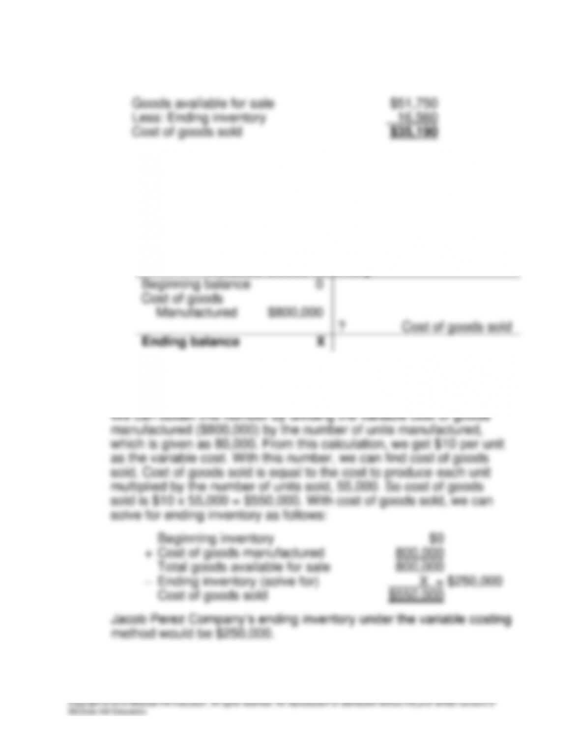
Requirement 3: Weighted average
For average cost, we divide goods available for sale by the units
available for sale. These totals come from the first table in our
solution. Specifically,
9-10
E9–9. Computing ending inventory and cost of sales under direct and
absorption costing (LO 4)
(AICPA adapted)
Requirement 1:
Finished goods inventory under variable (direct) costing.
Finished Goods Inventory
Beginning balance
0
Cost of goods
Manufactured
$800,000
?
Cost of goods sold
Ending balance
X
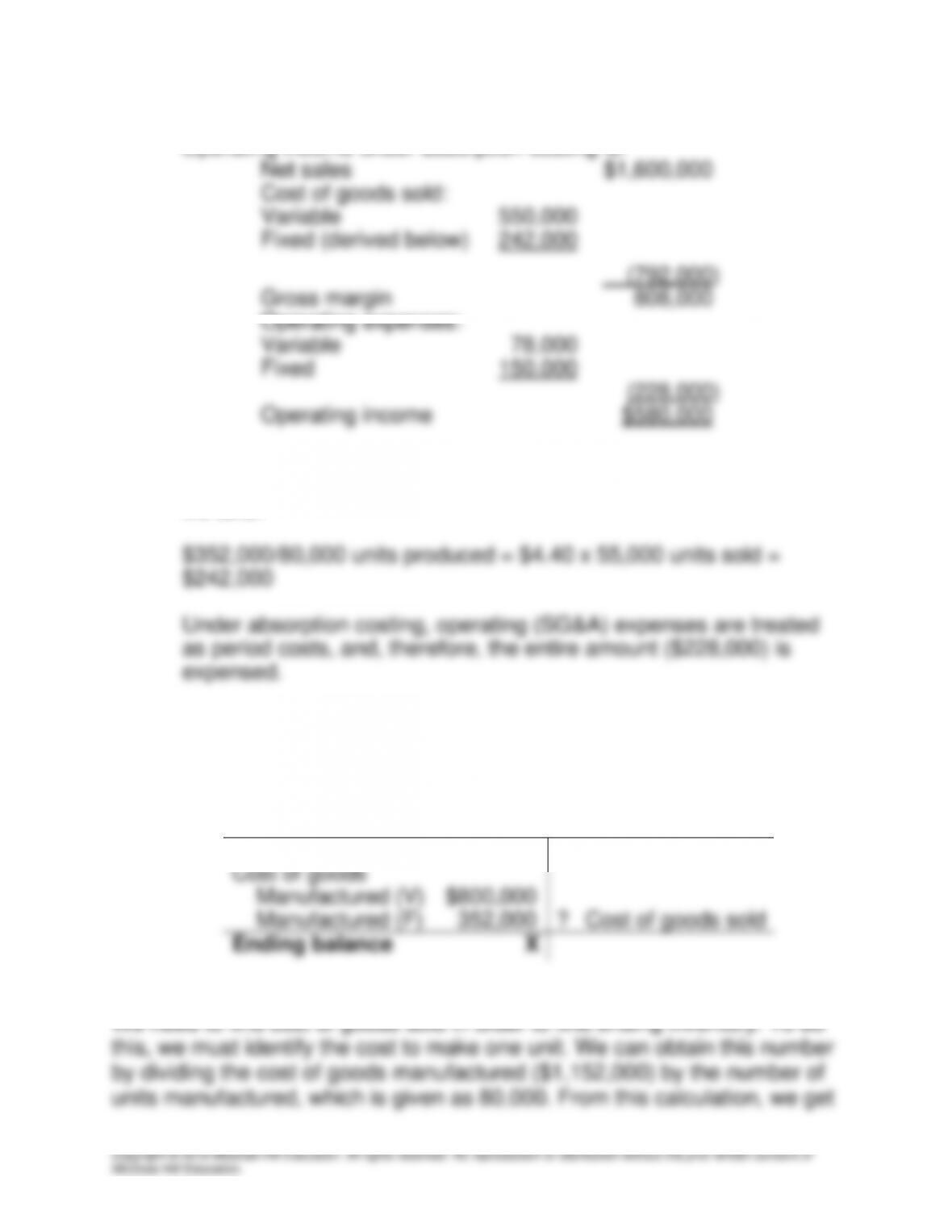
To begin, we know cost of goods manufactured and the beginning
balance. We need to find cost of goods sold in order to find ending
inventory. To do this, we must identify the cost to make one unit.
9-11
Requirement 2:
Operating income under absorption costing is:
Net sales
$1,600,000
Cost of goods sold:
Variable
550,000
Fixed (derived below)
242,000
(792,000)
Gross margin
808,000
Operating expenses:
Variable
78,000
Fixed
150,000
(228,000)
Operating income
$580,000
Absorption costing includes fixed manufacturing costs in inventory.
To find the fixed manufacturing cost portion of cost of goods sold,
we take:
Requirement 3:
Finished goods inventory and cost of goods sold under absorption
costing.
Finished Goods Inventory
Beginning balance
0
Cost of goods
Manufactured (V)
$800,000
Manufactured (F)
352,000
?
Cost of goods sold
Ending balance
X
To begin, we know cost of goods manufactured and the beginning balance.
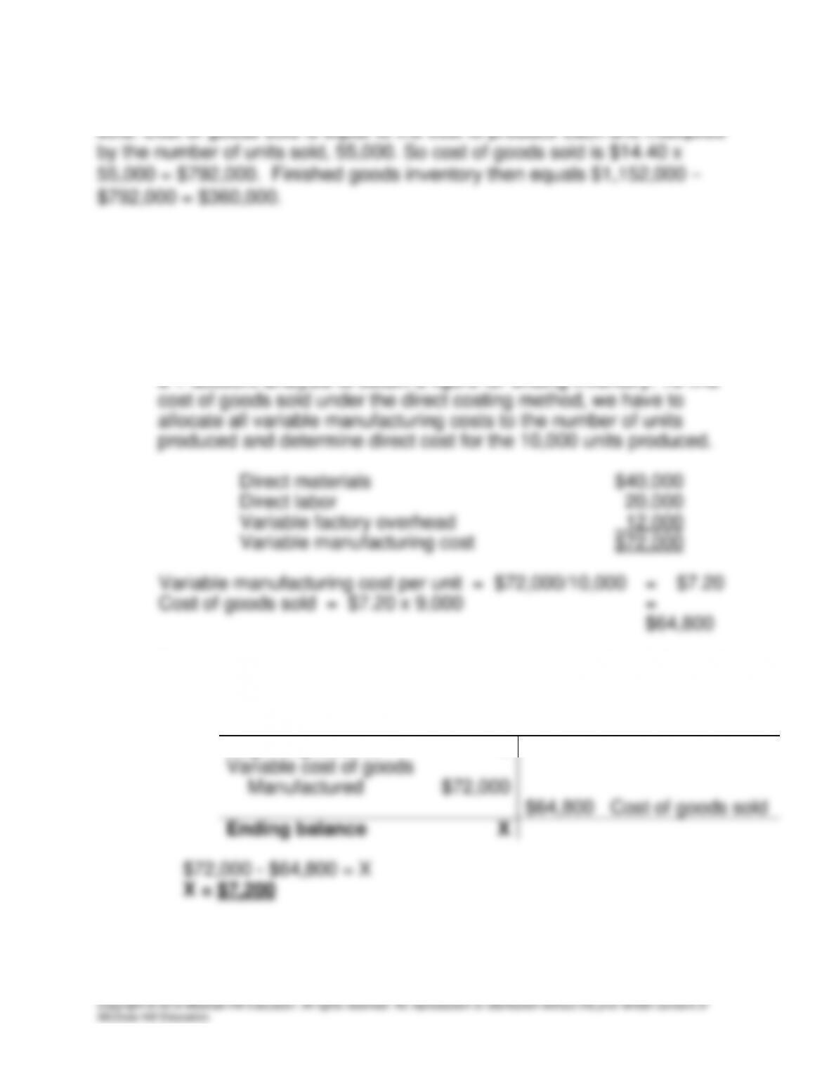
9-12
$14.40 per unit as the cost. With this number, we can find cost of goods
E9–10. Computing ending inventory and cost of goods sold under
absorption and variable costing (LO 4)
(AICPA adapted)
Requirement 1:
To find the cost of finished goods inventory at December 31, 2014,
we first need to find cost of goods sold for the year; then we will use
a T-account analysis to obtain a figure for ending inventory. To find
Now that we know cost of goods sold, we can analyze the finished
goods inventory T-account.
Finished Goods Inventory
Beginning balance
0
Variable cost of goods
Manufactured
$72,000
$64,800
Cost of goods sold
Ending balance
X
9-13
Requirement 2:
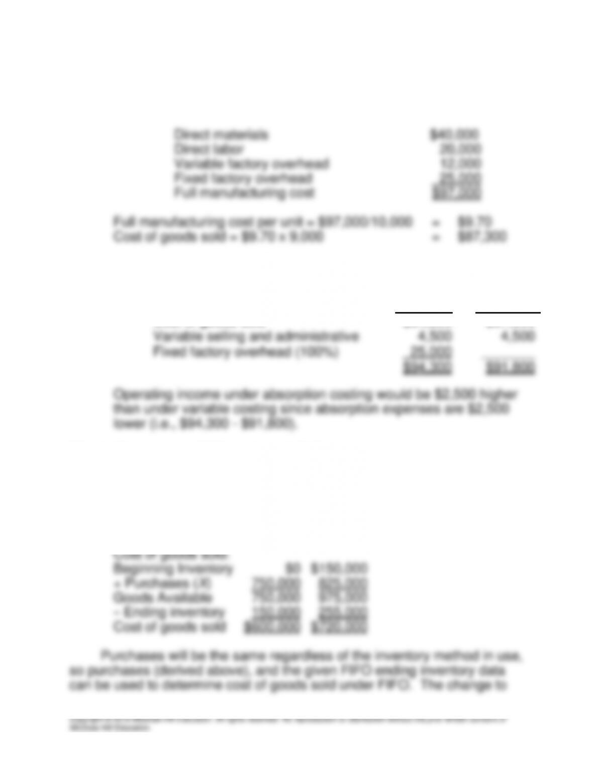
Cost of goods manufactured under absorption costing is computed
as follows:
Therefore, comparative total expense would be:
Variable
Costing_
Absorption
_Costing_
Cost of goods sold
$64,800
$87,300
Variable selling and administrative
4,500
4,500
Fixed factory overhead (100%)
_25,000
_______
$94,300
$91,800
E9–11. Changing to FIFO method (LO 5)
(AICPA adapted)
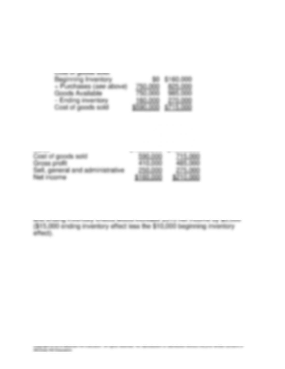
Use the given data (cost of goods sold, ending inventory) to derive
purchases, as indicated below:
Average Cost:
2014
2015
Cost of goods sold:
Beginning Inventory
$0
$150,000
+ Purchases (X)
750,000
825,000
Goods Available
750,000
975,000
− Ending inventory
150,000
255,000
Cost of goods sold
$600,000
$720,000
9-14
FIFO would affect the value of both the beginning and ending inventory in
2015. The specific calculations appear below:
FIFO:
2014
2015
Cost of goods sold:
Beginning Inventory
$0
$160,000
+ Purchases (see above)
750,000
825,000
Goods Available
750,000
985,000
− Ending inventory
160,000
270,000
Cost of goods sold
$590,000
$715,000
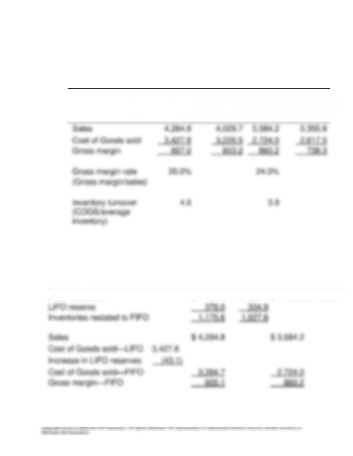
Having determined FIFO cost of goods sold, net income for 2015 under
FIFO can be calculated:
2014
2015
Sales
$1,000,000
$1,200,000
Cost of goods sold
590,000
715,000
Gross profit
410,000
485,000
Sell, general and administrative
250,000
275,000
Net income
$160,000
$210,000
Net income for 2015 is $5,000 higher than it would have been under
average cost. Although ending 2015 FIFO inventory is $15,000 higher,
which decreases cost of goods sold, beginning 2015 FIFO inventory is
$10,000 higher, which increases cost of goods sold. Netting the beginning
9-15
E9–12. Converting LIFO to FIFO (LO 6)
Requirement 1:
KW Steel Corp.
Waretown Steel
($ in millions)
2014
2013
2014
2013
Balance sheet
inventories
$ 797.6
$ 692.7
$ 708.2
$ 688.6
LIFO reserve
378.0
334.9
Sales
4,284.8
4,029.7
3,584.2
3,355.8
Cost of Goods sold
3,427.8
3,226.5
2,724.0
2,617.5
Gross margin
857.0
803.2
860.2
738.3
Gross margin rate
20.0%
24.0%
(Gross margin/sales)
Inventory turnover
4.6
3.9
(COGS/average
inventory)
A comparison of the ratios suggests that KW has a lower gross
margin than Waretown, but a better inventory turnover.
Requirement 2:
KW Steel Corp.
Waretown Steel
($ in millions)
2014
2013
2014
2013
Total inventories
$ 797.6
$ 692.7
$ 708.2
$ 688.6
LIFO reserve
378.0
334.9
Inventories restated to FIFO
1,175.6
1,027.6
Sales
$ 4,284.8
$ 3,584.2
Cost of Goods sold—LIFO 3,427.8
Increase in LIFO reserves (43.1)
Cost of Goods sold—FIFO
3,384.7
2,724.0
Gross margin—FIFO
900.1
860.2