Chapter 05 – Lecture Notes
5-1
Chapter 5 Lecture Notes
Chapter theme: Cost-volume-profit (CVP) analysis helps
managers understand the interrelationships among cost,
volume, and profit by focusing their attention on the
interactions among the prices of products, volume of
activity, per unit variable costs, total fixed costs, and
mix of products sold. It is a vital tool used in many
business decisions such as deciding what products to
manufacture or sell, what pricing policy to follow, what
marketing strategy to employ, and what type of productive
facilities to acquire.
I. Assumptions of CVP analysis
A. Four key assumptions underlie CVP analysis:
i. Selling price is constant.
ii. Costs are linear and can be accurately divided into
variable and fixed elements. The variable element
is constant per unit, and the fixed element is
constant in total over the entire relevant range.
iii. In multiproduct companies, the sales mix is
constant.
iv. In manufacturing companies, inventories do not
change. The number of units produced equals the
number of units sold.
Helpful Hint: Point out that nothing is sacred about
these assumptions. When violations of these
assumptions are significant, managers can and do
modify the basic CVP model. Spreadsheets allow
1
2
Chapter 05 – Lecture Notes
5-2
practical models that incorporate more realistic
assumptions. For example, nonlinear cost functions
with step fixed costs can be modeled using “If…Then”
functions.
II. The basics of cost-volume-profit (CVP) analysis
Learning Objective 1: Explain how changes in activity
affect contribution margin and net operating income.
A. The contribution income statement is helpful to
managers in judging the impact on profits of changes in
selling price, cost, or volume. For example, let’s look at
a hypothetical contribution income statement for
Racing Bicycle Company (RBC). Notice:
i. The emphasis is on cost behavior. Variable costs
are separate from fixed costs.
ii. The contribution margin is defined as the amount
remaining from sales revenue after variable
expenses have been deducted.
iii. Contribution margin is used first to cover fixed
expenses. Any remaining contribution margin
contributes to net operating income.
5
4
3
Chapter 05 – Lecture Notes
5-3
iv. Sales, variable expenses, and contribution margin
can also be expressed on a per unit basis. Thus:
1. For each additional unit RBC sells, $200
more in contribution margin will help to
cover fixed expenses and provide a profit.
2. Notice, each month RBC must generate at
least $80,000 in total contribution margin to
break-even (which is the level of sales at
which profit is zero).
3. Therefore, if RBC sells 400 units a month, it
will be operating at the break-even point.
4. If RBC sells one more bike (401 bikes), net
operating income will increase by $200.
v. You do not need to prepare an income statement to
estimate profits at a particular sales volume. Simply
multiply the number of units sold above break-even
by the contribution margin per unit.
1. For example, if RBC sells 430 bikes, its net
operating income will be $6,000.
B. CVP relationships in equation form (for those who
prefer an algebraic approach to solving problems in the
chapter)
i. The contribution format income statement can be
expressed in equation form as shown on this slide.
1. This equation can be used to show the profit
RBC earns if it sells 401 bikes. Notice, the
answer of $200 mirrors our earlier solution.
6
7
8
9
10
11
12
Chapter 05 – Lecture Notes
5-4
ii. When a company has only one product we can
further refine this equation as shown on this slide.
1. This equation can also be used to show the
$200 profit RBC earns if it sells 401 bikes.
iii. The profit equation can also be expressed in terms
unit contribution margin as shown on this slide.
1. This equation can also be used to compute
RBC’s $200 profit if it sells 401 bikes.
Learning Objective 2: Prepare and interpret a cost–
volume-profit (CVP) graph and a profit graph.
C. CVP relationships in graphic form
i. The relationships among revenue, cost, profit, and
volume can be expressed graphically by preparing a
cost-volume-profit (CVP) graph. To illustrate, we
will use contribution income statements for RBC at
0, 200, 400, and 600 units sold.
Helpful Hint: Mention to students that the graphic form
of CVP analysis may be preferable to them if they are
uncomfortable with algebraic equations.
ii. In a CVP graph, unit volume is represented on the
horizontal (X) axis and dollars on the vertical (Y)
axis. A CVP graph can be prepared in three steps.
1. Draw a line parallel to the volume axis to
represent total fixed expenses.
2. Choose some sales volume (e.g., 400 units)
and plot the point representing total
18
19
20
21
17
15
14
16
13
Chapter 05 – Lecture Notes
5-5
expenses (e.g., fixed and variable) at that sales
volume. Draw a line through the data point
back to where the fixed expenses line
intersects the dollar axis.
3. Choose some sales volume (e.g., 400 units)
and plot the point representing total sales
dollars at the chosen activity level. Draw a
line through the data point back to the
origin.
iii. Interpreting the CVP graph.
1. The break-even point is where the total
revenue and total expense lines intersect.
2. The profit or loss at any given sales level is
measured by the vertical distance between
the total revenue and the total expense lines.
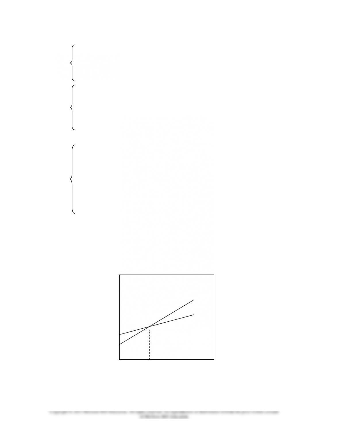
Helpful Hint: Ask students what the CVP graph would
look like for a public agency like a county hospital
receiving a fixed budget each year and collecting fees
less than its variable costs. It would look like this:
This is the reverse of the usual situation. If such an
organization has volume above the break-even point, it
will experience financial difficulties.
22
23
Total
expenses
Total
revenue
21
Chapter 05 – Lecture Notes
5-6
iv. An even simpler form of the CVP graph is called
the profit graph. The profit graph is based on the
equation shown on this slide.
1. To plot the graph, compute the profit at two
different sales volumes, plot the points, and
then connect them with a straight line. This
slide contains the profit graph for RBC.
Notice:
a. The sales volumes plotted on this
graph are 300 and 500 bikes.
b. The breakeven point is 400 bikes.
D. Contribution margin ratio (CM ratio)
Learning Objective 3: Use the contribution margin
ratio (CM ratio) to compute changes in contribution
margin and net operating income resulting from
changes in sales volume.
i. The CM ratio is calculated by dividing the total
contribution margin by total sales.
1. For RBC, the CM ratio is 40%. Thus, each
$1.00 increase in sales results in a total
contribution margin increase of 40¢.
ii. The CM ratio can also be calculated by dividing the
contribution margin per unit by the selling price
per unit.
1. For RBC the CM ratio is 40%.
2. If RBC increases sales from 400 to 500
bikes, the increase in contribution margin
($20,000) can be calculated by multiplying
27
28
29
26
25
24
Chapter 05 – Lecture Notes
5-7
3. the increase in sales ($50,000) by the CM
ratio (40%).
Quick Check – contribution margin ratio
iii. The relation between profit and the CM ratio can
also be expressed in terms of the equation shown
on this slide.
1. For example, we can use this equation to
calculate RBC’s profit of $20,000 at a
volume of 500 bikes.
E. Applications of CVP concepts
Learning Objective 4: Show the effects on net operating
income of changes in variable costs, fixed costs, selling
price, and volume.
Helpful Hint: The five examples that are forthcoming
should indicate to students the range of uses of CVP
analysis. In addition to assisting management in
determining the level of sales that is needed to break–
even or generate a certain dollar amount of profit, the
examples illustrate how the results of alternative
decisions can be quickly determined.
i. The variable expense ratio
1. Before proceeding with five examples that
demonstrate various applications of CVP
concepts, we need to define the variable
expense ratio as the ratio of variable
expenses to sales.
30-31
34
33
32
29
Chapter 05 – Lecture Notes
5-8
ii. Change in fixed cost and sales volume
1. What is the profit impact if RBC can
increase unit sales from 500 to 540 by
increasing the monthly advertising budget
by $10,000?
a. Preparing a contribution income
statement reveals a $2,000 decrease in
profits.
b. A shortcut solution using incremental
analysis also reveals a $2,000 decrease
in profits.
iii. Change in variable costs and sales volume.
1. What is the profit impact if RBC can use
higher quality raw materials, thus increasing
variable costs per unit by $10, to generate an
increase in unit sales from 500 to 580?
a. The contribution income statement
reveals a $10,200 increase in profits.
iv. Change in fixed cost, sales price, and sales
volume.
1. What is the profit impact if RBC: (1) cuts its
selling price $20 per unit, (2) increases its
advertising budget by $15,000 per month,
and (3) increases unit sales from 500 to 650
units per month?
a. The contribution income statement
reveals a $2,000 increase in profits.
36
37
38
39
40
41
35