Chapter 18 Cost Behavior and Cost-Volume-Profit Analysis
Chapter 18
Cost Behavior and
Cost-Volume-Profit Analysis
Related Assignment Materials
Student Learning Objectives
Discussion
Questions
Quick
Studies*
Exercises*
Problems*
Beyond the
Numbers
Conceptual objectives:
C1. Describe different types of cost
behavior in relation to
production and sales volume.
1, 2, 3, 4, 5,
10, 12, 16, 19,
21
18-1, 18-2
18-2, 18-3,
18-4
18–18
RIA, EC,
TTN, ED
C2. Describe several applications
of cost-volume-profit analysis.
11, 15
18-7, 18-10
18-5, 18-12,
18-13, 18-14,
18-15, 18-16
18-4, 18-5
CIP, TIA
Analytical objectives:
A1. Compute contribution margin
and describe what it reveals
about a company’s cost
structure.
6, 7, 8, 9
18-5, 18-14
18-1, 18-4,
18-5, 18-6
ED
A2. Analyze changes in sales using
the degree of operating
leverage.
17, 18
18–11
18-9, 18-21
CA
Procedural objectives:
P1. Determine cost estimates using
the scatter diagram, high-low
method and regression
methods of estimating costs.
13
18-3, 18-4
18-1, 18-6,
18-7, 18-8
18-3
P2. Compute break-even point for a
single product company.
14
18-6, 18-8,
18-9
18–10
18-2, 18-4,
18-6
CA
P3. Graph costs and sales for a
single product company.
20
18–13
18–11
18-2
P4. Compute break-even point for a
multiproduct company.
20
18–12
18-17, 18-18,
18–19, 18-20
18-5, 18-7
HTR, GD
*See additional information on next page that pertains to these quick studies, exercises and problems.
Chapter 18 Cost Behavior and Cost-Volume-Profit Analysis
website, in whole or part. 18-2
Additional Information on Related Assignment Material
Assignment materials that can be completed by students using:
Sage 50 and QuickBooks Pro 2013 templates — none
Excel templates. Problems 18-2A and 18-6A
** The Serial Problem for Success Systems, which covers numerous learning objectives, can be
the chapters. Even if previous segments were not assigned, students can begin the segment of the
serial problem that is included in this chapter. It is most readily solved if students use the Working
Papers that accompany the book.).
Synopsis of Chapter Revision
• Leather Head Sports: NEW opener with new entrepreneurial assignment
• Was Chapter 22 in prior edition
• New graphics on relations between per-unit fixed and variable costs and volume
• Revised discussion of per-unit fixed and variable costs
• Moved discussion of margin of safety to section on break-even
• Revised discussion of assumptions in CVP analysis
• Enhanced the formatting and layout of several key exhibits
• New discussion and examples of using the contribution margin income statement to perform
sensitivity analyses and compute sales needed for target income
• Revised data for estimating cost behavior
• New discussion on the use of RFID tags to control inventory costs and for error-reduction
PowerPoint® Show Slides
Chapter Learning Objective
PowerPoint® Slides
C1
6-13
P1
14-18
P2
19, 22-25
A1
20-21
P3
26-27
C2
28-33
P4
34-35
A2
36
Chapter 18 Cost Behavior and Cost-Volume-Profit Analysis
Chapter Outline
I. Identifying Cost Behavior (CVP analysis) ⎯Cost-volume-profit
analysis is a tool to predict how changes in costs and sales levels
affect income. CVP analysis involves computing the sales level at
which a company neither earns an income nor incurs a loss, called the
break-even point. Basic form of CVP analysis is called break-even
analysis. Conventional CVP analysis requires that all costs must be
classified as either fixed or variable with respect to production or sales
volume.
A. Fixed Costs
1. A fixed cost remains unchanged in amount when volume of
activity varies from period to period within a relevant range.
Total fixed cost does not change.
2. On a per unit basis, as the level of production changes the
fixed cost per unit of output decreases as volume increases
(and vice versa).
3. When production volume and cost are graphed, units of
product are usually plotted on the horizontal axis and dollars
of cost are plotted on the vertical axis.
(cost remains constant at all levels of volume within the
relevant range).
cost amount.
4. Likely that amount of fixed cost will change when outside of
relevant range.
production.
3. When production volume and cost are graphed:
the zero cost level.
b. The straight line is upward (positive) sloping. The line
rises as volume increases.
C. Mixed Costs
2. When volume and cost graphed:
a. Mixed cost is represented by a straight line with an
Notes
Chapter 18 Cost Behavior and Cost-Volume-Profit Analysis
website, in whole or part. 18-4
Chapter Outline
when volume is zero) on cost (vertical) axis. As activity level
increases, mixed cost line increases at an amount equal to the
variable cost per unit.
3. Mixed costs are often separated into fixed and variable
components when included in a CVP analysis.
D. Step-wise Costs
1. Fixed within a relevant range of the current production
volume. If production volume expands significantly, total
costs go up by a lump-sum amount (stair-step cost).
2. Treated as either fixed or variable cost in conventional CVP
analysis; depends on width of range, and requires judgment.
1. A linear cost increases at a constant rate as volume of activity
increases.
as a curved line that starts at intersection point of cost axis and
volume axis (total cost is zero when volume is zero) and
II. Measuring Cost Behavior⎯After establishing that cost data are
reliable and useful in predicting future costs, three methods are
commonly used to analyze past cost behavior.
2. Units are plotted on the horizontal axis and cost is on the
vertical axis.
3. Each point reflects the cost and number of units for a prior
points visually.
a. Intersection point of line on cost (vertical) axis is at fixed
cost amount.
b. The variable cost per unit of volume equals the slope of
the line.
i. Select any two points on horizontal axis.
ii. Draw a vertical line from each of these points to
intersect the estimated line of cost behavior.
iii. Compute the slope of the line, or variable cost, as the
change in cost divided by the change in units.
c. Cost equation.
i. Fixed cost plus (variable cost per unit times number of
units of volume).
Notes
Chapter 18 Cost Behavior and Cost-Volume-Profit Analysis
Chapter Outline
ii. Useful to predict future cost levels at different volumes.
5. Deficiency of scatter diagram method⎯estimates are based on
“visual fit” of cost line, subject to interpretation.
B. High-low Method
1. Estimate of the cost equation determined by graphically
connecting the two cost amounts at the highest and lowest unit
volumes.
a. Intersection point of line on cost axis is at fixed cost
amount.
b. Variable cost per unit is the slope of the line⎯computed
as “change in cost” (difference between cost at the highest
number of units and cost at the lowest number of units)
divided by “change in sales” (difference between the
highest and lowest unit volumes).
2. Cost equation may differ slightly from that determined using
advanced cost accounting courses.
1. Statistical method of identifying cost behavior.
2. Cost equation readily calculated using most spreadsheet
programs or calculators.
3. Cost equation may differ slightly from those determined using
the scatter diagram and high-low methods; superior due to use
of all data points available.
D. Comparison of Cost Estimation Methods—all three methods use
past data, so their cost estimates are only as good as the data used
for estimation. The more data points used in regression or scatter
diagram methods should yield more accurate estimates than the
high-low method.
III. Using Break-Even Analysis⎯special case of CVP analysis.
A. Contribution margin and its measures
1. After costs are classified as either fixed or variable, we can
compute a product’s contribution margin.
2. Unit contribution margin is the amount a product’s unit
selling price exceeds its total variable cost per unit.
3. Excess amount contributes to covering fixed costs and
generating profits on a per unit basis.
4. Contribution margin per unit = sales price per unit – total
variable cost per unit.
Notes
Chapter 18 Cost Behavior and Cost-Volume-Profit Analysis
Chapter Outline
5. Contribution margin ratio is the percent of a unit’s selling
price that exceeds total unit variable cost.
6. Contribution margin ratio = unit. contribution margin divided
by selling price per unit.
B. Computing Break-Even Point
1. Break-even point
a. Sales level at which neither a profit or loss is incurred.
b. Expressed either in units or dollars of sales.
c. Shows whether sales will at least cover total costs.
C. Computing the Margin of Safety
1. Margin of safety equals excess of expected sales over sales at
percent of predicted level of sales (percent equals margin of
safety divided by expected sales).
1. Horizontal axis⎯is the number of units produced and sold.
2. Vertical axis⎯dollars of sales and costs.
3. Three steps:
a. Plot fixed costs on vertical axis; draw horizontal line at
costs) for a relevant range of volume levels.
i. Line starts at fixed costs on vertical axis.
ii. Slope equals variable cost per unit; compute total
costs for any sales level, and connect this point with
the vertical axis intercept. Stop line at productive
capacity for the planning period.
c. Draw sales line.
i. Line starts at origin (zero units and zero dollars of
Notes
Chapter 18 Cost Behavior and Cost-Volume-Profit Analysis
website, in whole or part. 18-7
Chapter Outline
a. Volume levels to left of break-even point⎯vertical
distance is amount of loss expected because the total costs
line is above the total sales line.
b. Volume levels to right of break-even point⎯vertical
distance is amount of profit expected because the total
sales line is above the total costs line.
E. Making Assumptions in Cost-Volume-Profit Analysis
1. CVP analysis assumes that selling prices per unit, variable
costs per unit and total fixed costs are all held constant.
2. Working with Assumptions: if the expected cost and sales
behavior differ from these assumptions the results of CVP
analysis can be limited.
a. Summing costs can offset individual
deviations⎯individual variable cost items may not be
perfectly variable, but when summed, individual
deviations can offset each other.
b. CVP is applied to a relevant range of operations⎯to
assume a specific cost is variable or fixed is more likely
valid when operations are within the relevant range.
Relevant range of operations is the normal operating
can be increased without impacting costs, break-even
decreases. When selling prices decrease and the company
cannot reduce costs, break-even increases. Increases in
be reduced and selling prices held constant, break-even
decreases.
IV. Applying Cost-Volume-Profit Analysis ⎯useful in helping
managers evaluate likely effects of strategies considered in planning
business operations.
A. Computing Income from Sales and Costs – pretax income equals
sales less variable costs less fixed costs.
B. Computing Sales for a Target Income – sales (in dollars) required
for target after-tax income equals (fixed costs plus target after-tax
income) divided by CM ratio.
Notes
Chapter 18 Cost Behavior and Cost-Volume-Profit Analysis
Chapter Outline
C. Using Sensitivity Analysis⎯Knowing the effects of changing
some estimates used in CVP analysis by substituting new
estimated amounts (in total or per unit as appropriate) in the
related formula can be helpful in making predictions.
D. Computing Multiproduct Break-Even Point⎯Modify basic CVP
analysis when company produces and sells several products.
1. Important assumption⎯sales mix of different products is
known and remains constant.
2. Sales mix is the ratio (proportion) of the sales volumes for
various products.
expected sales mix.
a. Determine sales mix of various products.
b. Using sales mix, determine the selling price of a
composite unit by multiplying the sales mix ratio times the
selling price of each product and then adding the totals for
all of the products.
c. Compute the variable cost of a composite unit in the same
manner, and then determine the CM per composite unit.
d. Break-even point in composite units equals total fixed
costs divided by CM per composite unit.
f. Instead of computing contribution margin per composite
unit, a company can compute a weighted-average
contribution margin.
V. Decision Analysis—Degree of Operating Leverage⎯Useful tool in
assessing the effect of changes in the level of sales on income.
A. Operating leverage is the extent, or relative size, of fixed costs in
dollars) divided by pretax income.
C. Use DOL to measure the effect of changes in the level of sales on
pretax income by multiplying DOL by the percentage change in
sales.
Notes
Chapter 18 Cost Behavior and Cost-Volume-Profit Analysis
Chapter Outline
VI. Appendix 18A. Using Excel to Estimate Least Squares Regression.
Microsoft Excel and other spreadsheet software can be used to perform
least squares regressions to identify cost behavior.
In Excel, the INTERCEPT and SLOPE functions are used.
Spreadsheet software is useful in understanding cost behavior when
many data points are available.
Excel can also be used to create scatter diagrams. Excel will precisely
fit the regression line.
Notes

Chapter 18 Cost Behavior and Cost-Volume-Profit Analysis
website, in whole or part. 18–10
Chapter 18 – Alternate Demonstration Problem #1
Trimble Company sells an electronic toy for $40. The variable cost is $24
per unit and the fixed cost is $32,000 per year. Management is considering
the following changes:
Alternative #1
Lease a new packaging machine for $4,000 per year, which will reduce
variable cost by $1 per unit.
Alternative #2
Increase selling price 10 percent to counteract an expected 25 percent
increase in fixed cost.
Alternative #3
Reduce fixed cost by 25 percent by moving to a lower rent location. This
would have the effect of increasing variable costs by 10 percent.
Required:
Consider and answer each of the following questions independently:
(a) Determine the current break-even point in units and dollars.
(b) Determine the expected profit assuming alternative #1 and sales of
3,200 units.
(c) Determine the break-even point in units and dollars assuming
alternative #2.
(d) Determine the break-even point required in units and dollars
assuming alternative #3.
(e) Determine the volume of sales required to earn $23,600 assuming
alternative #3.
Chapter 18 Cost Behavior and Cost-Volume-Profit Analysis
website, in whole or part. 18–11
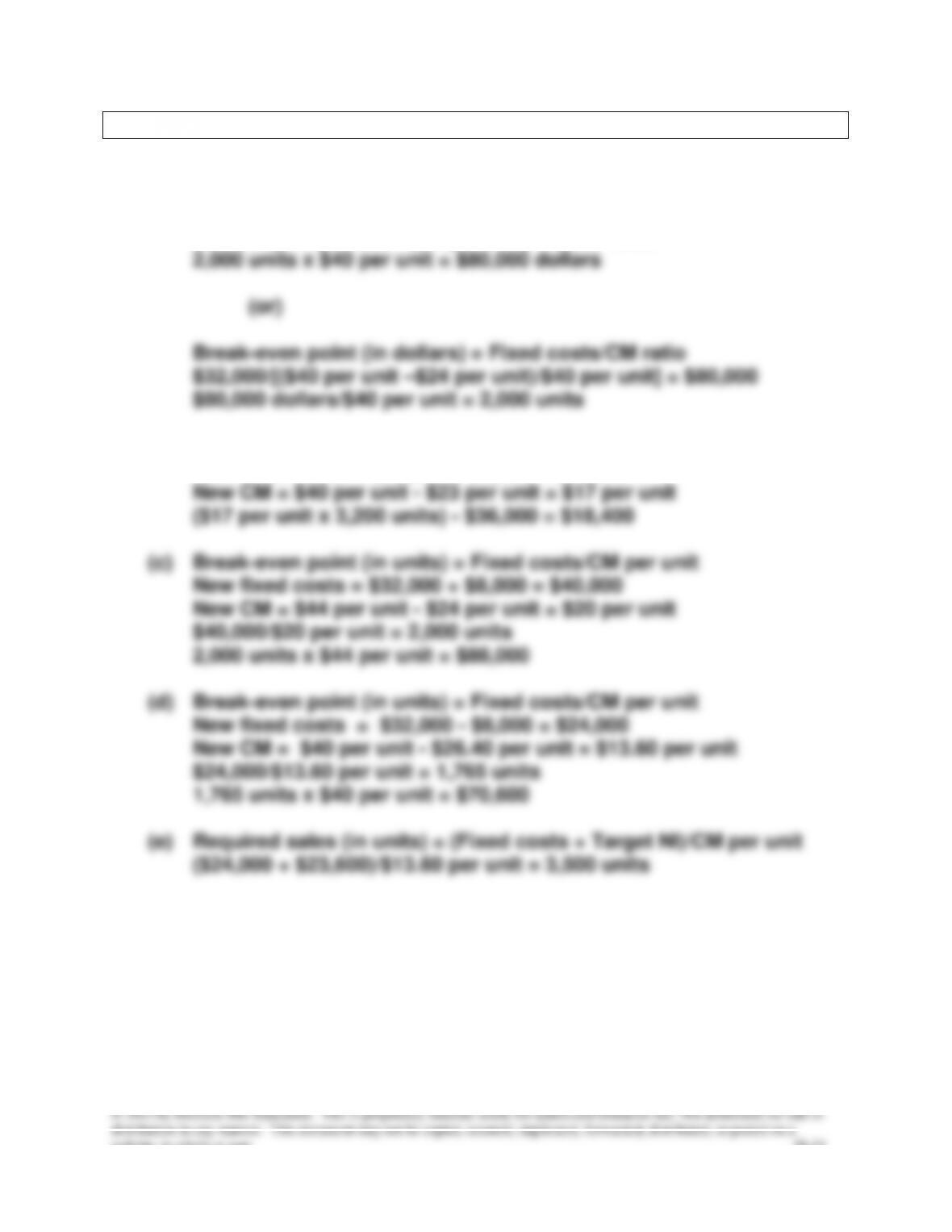
Solution: Chapter 18 Alternate Demonstration Problem #1
(a)
Break-even point (in units) = Fixed costs/CM per unit
$32,000/($40 per unit – $24 per unit) = 2,000 units
2,000 units x $40 per unit = $80,000 dollars
(or)
Break-even point (in dollars) = Fixed costs/CM ratio
$32,000/[($40 per unit –$24 per unit)/$40 per unit] = $80,000
$80,000 dollars/$40 per unit = 2,000 units
(b)
Net income = (CM per unit x number of units sold) – Fixed costs
New fixed costs = $32,000 + $4,000 = $36,000
New CM = $40 per unit – $23 per unit = $17 per unit
($17 per unit x 3,200 units) – $36,000 = $18,400
(c)
Break-even point (in units) = Fixed costs/CM per unit
New fixed costs = $32,000 + $8,000 = $40,000
New CM = $44 per unit – $24 per unit = $20 per unit
$40,000/$20 per unit = 2,000 units
2,000 units x $44 per unit = $88,000
(d)
Break-even point (in units) = Fixed costs/CM per unit
New fixed costs = $32,000 – $8,000 = $24,000
New CM = $40 per unit – $26.40 per unit = $13.60 per unit
$24,000/$13.60 per unit = 1,765 units
1,765 units x $40 per unit = $70,600
(e)
Required sales (in units) = (Fixed costs + Target NI)/CM per unit
($24,000 + $23,600)/$13.60 per unit = 3,500 units