Chapter 17 – Additional Topics in Variance Analysis
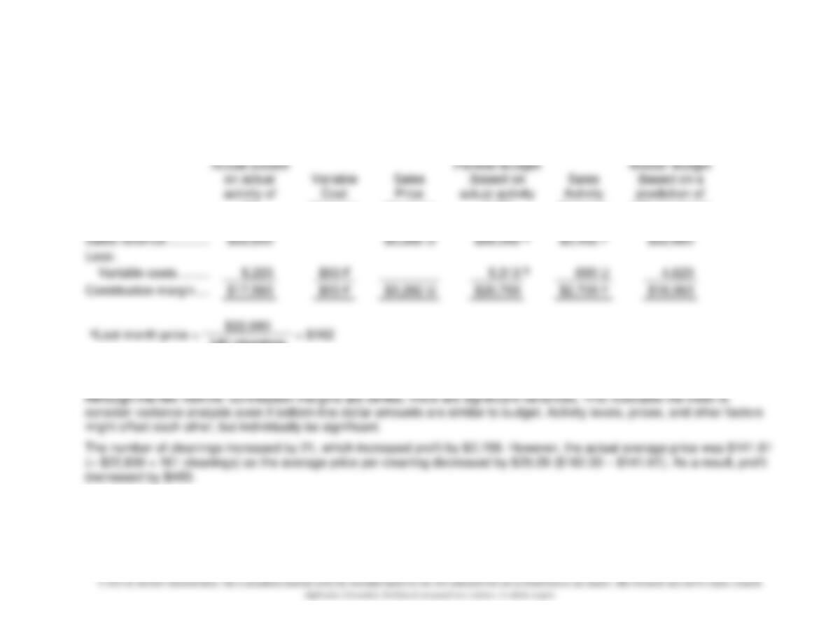
17–41. (20 min.) Derive Amounts for Profit Variance Analysis: Aqua Clean, Inc.
Hint: Use last month’s actual as master budget.
Actual (based
on actual
activity of
161
cleanings)
Variable
Cost
Variance
Sales
Price
Variance
Flexible Budget
(based on
actual activity
of 161
cleanings)
Sales
Activity
Variance
Master Budget
(based on a
prediction of
140 cleanings)
Sales revenue ………….……………….
$22,800
$3,282 U
$26,082
a
$3,402 F
$22,680
Less:
Variable costs ……….………………….
5,220
$93 F
5,313
b
693 U
4,620
Contribution margin …..………………………
$17,580
$93 F
$3,282 U
$20,769
$2,709 F
$18,060
aLast month price =
$22,680
= $162
140 cleanings
$26,082 = $162 x 161 cleanings
bLast month unit variable cost = $4,620 ÷ 140 cleanings = $33; $5,313 = $33 x 161 cleanings.
Chapter 17 – Additional Topics in Variance Analysis
17–30
17–42. (20 min.) Flexible budget: Oak Hill Township.
Flexible budget is based on actual activity of 94,500 miles for costs that vary per mile.
a. $8,505; $10 over budget.
$6,750 x (94,500 miles ÷ 75,000 miles) = $8,505
Chapter 17 – Additional Topics in Variance Analysis
17–31
Solutions to Case
17–43. Comprehensive Overview of Budgets and Variances Racketeer, Inc.
The following solution is based on a report by Tom Terpstra.
Elmo’s problem is that he thinks that the graph and the income statement measure the
same thing. Otto should have told him that they do not. The income statement presents
actual costs in a full-absorption costing format, while the profit graph is based on standard
actual profit would differ from the profit on the graph. These variances are:
Material ……………………………….…………………….
$490
U
Labor …………………………………..…………………..
392
U
Overhead …………………………….…………………….
190
U
Selling and administrative …………………………..
300
F
Total ……………………………………………………….
$772
U
The other part of the difference between the two profit figures is explained by the
difference in accounting methods. Variable costing expenses fixed costs when they are
incurred. With full-absorption, the fixed costs are assigned to the units produced, and then
expensed in the period in which the units are sold. Racketeer treats each racket as having
a fixed cost of $0.47. For the 10,000 rackets sold, the fixed cost expense is $4,700 under
$1,410.
Chapter 17 – Additional Topics in Variance Analysis
17–32
17–43. (continued)
Now the two results can be reconciled:
Profit per chart …………………………..…………….….
$20,940
Less:
Cost variances ……………………………………..….
772
Additional fixed costs in full-absorption …….….
1,410
Profit per Income Statement ………………………….
$18,758
Besides failing to explain the profit graph, Otto also failed to set up a format to take
advantage of the standards he developed. The company should set up a chart showing
the actual results, the flexible budget, and the master budget. This would provide
information concerning the profit changes in relation to the change in sales volume.
Additionally, the manufacturing variances could be analyzed in greater detail, as shown in
Exhibits A and B on the following pages.
Chapter 17 – Additional Topics in Variance Analysis
17–33
17–43. (continued)
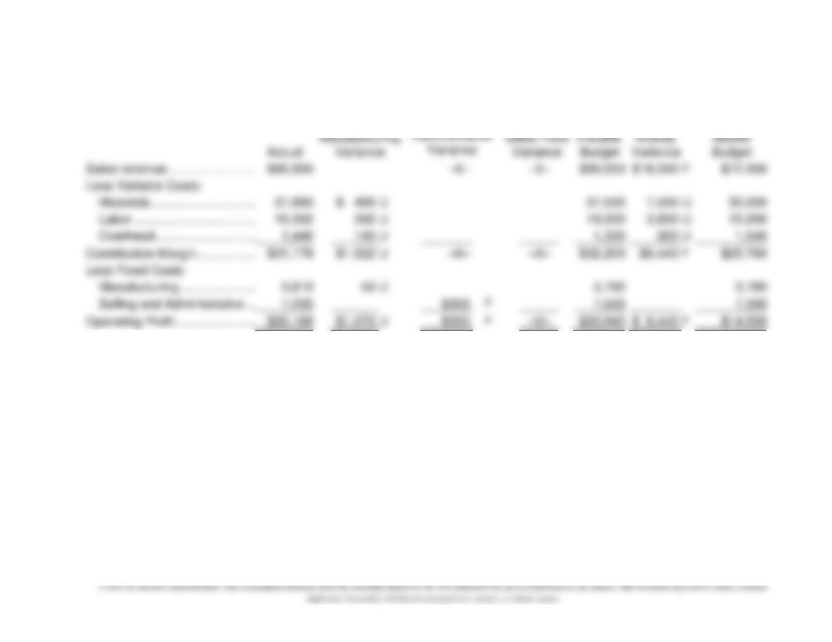
Exhibit A Comparison of Master Budget to Actual Results.
Actual
Manufacturing
Variance
Selling and
Administrative
Variance
Sales Price
Variance
Flexible
Budget
Activity
Variance
Master
Budget
Sales revenue ……………………..
$90,000
–0–
–0–
$90,000
$18,000
F
$72,000
Less Variable Costs:
Materials ………………………….
37,990
$ 490
U
37,500
7,500
U
30,000
Labor ……………………………...
19,392
392
U
19,000
3,800
U
15,200
Overhead ………………………...
1,440
140
U
1,300
260
U
1,040
Contribution Margin ……………...
$31,178
$1,022
U
–0–
–0–
$32,200
$6,440
F
$25,760
Less Fixed Costs:
Manufacturing …………………..
3,810
50
U
3,760
3,760
Selling and Administrative ….
7,200
$300
F
7,500
7,500
Operating Profit …………………...
$20,168
$1,072
U
$300
F
–0–
$20,940
$ 6,440
F
$14,500
Chapter 17 – Additional Topics in Variance Analysis
17–34
17–43. (continued)
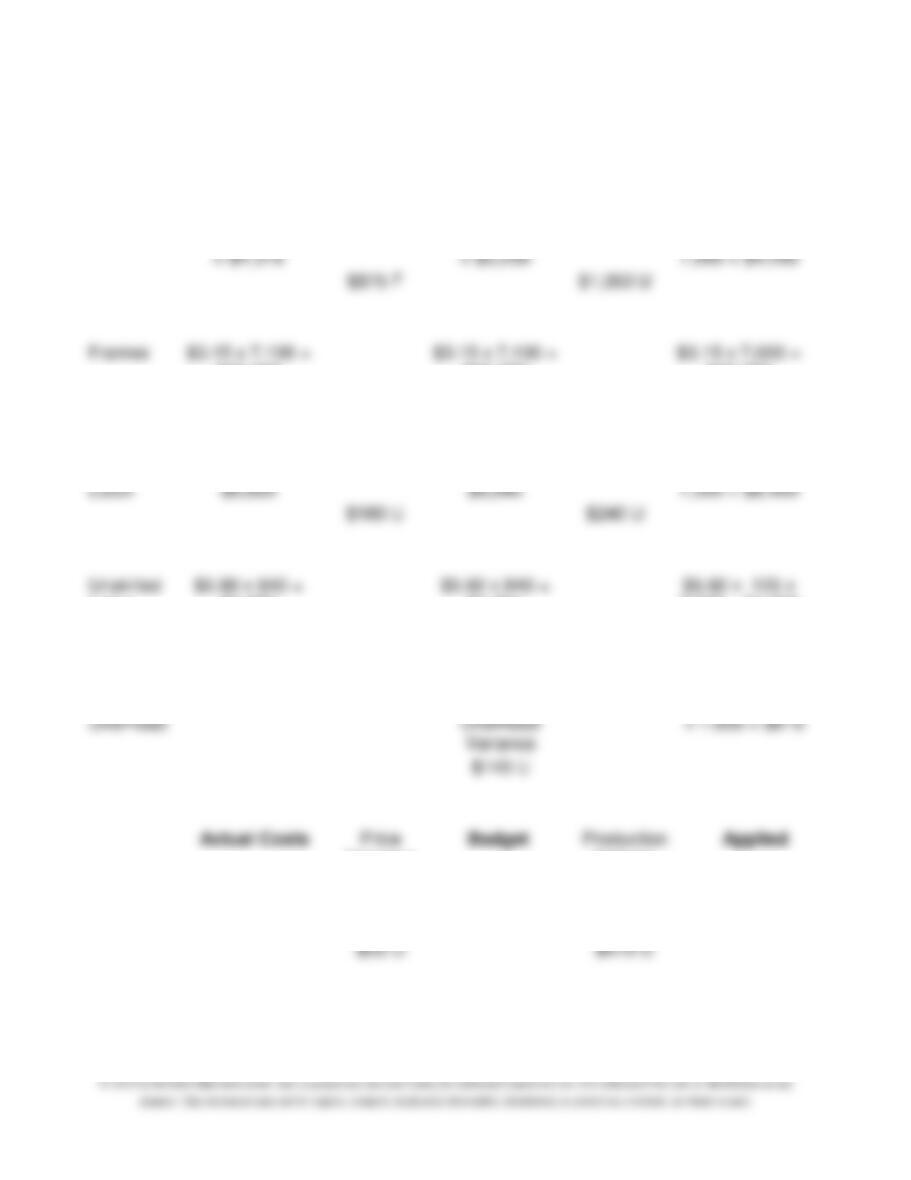
Exhibit B Manufacturing Cost Variances.
Actual Costs
Price
Variance
Actual Inputs
at Standard
Price
Efficiency
Variance
Flexible Budget
String
$0.025 x 175,000
= $4,375
$0.03 x 175,000
= $5,250
$0.03 x 20 x
7,000 = $4,200
$875 F
$1,050 U
Frames
$3.15 x 7,100 =
$22,365
$3.15 x 7,100 =
$22,365
$3.15 x 7,000 =
$22,050
$-0-
$315 U
Skilled
Labor
$9.80 x 900 =
$8,820
$9.60 x 900 =
$8,640
$9.60 x .125 x
7,000 = $8,400
$180 U
$240 U
Unskilled
Labor
$5.80 x 840 =
$4,872
$5.60 x 840 =
$4,704
$5.60 x .125 x
7,000 = $4,900
$168 U
$196 F
Variable
Overhead
$1,050
Total Variable
Overhead
Variance
($0.10 + $.03)
x 7,000 = $910
$140 U
Actual Costs
Price
Variance
Budget
Production
Volume
Variance
Applied
Fixed
Overhead
$3,810
$0.47 x 8,000 =
$3,760
($0.47 x 7,000)
= $3,290
$50 U
$470 U
Chapter 17 – Additional Topics in Variance Analysis
17–35
17–43. (continued)
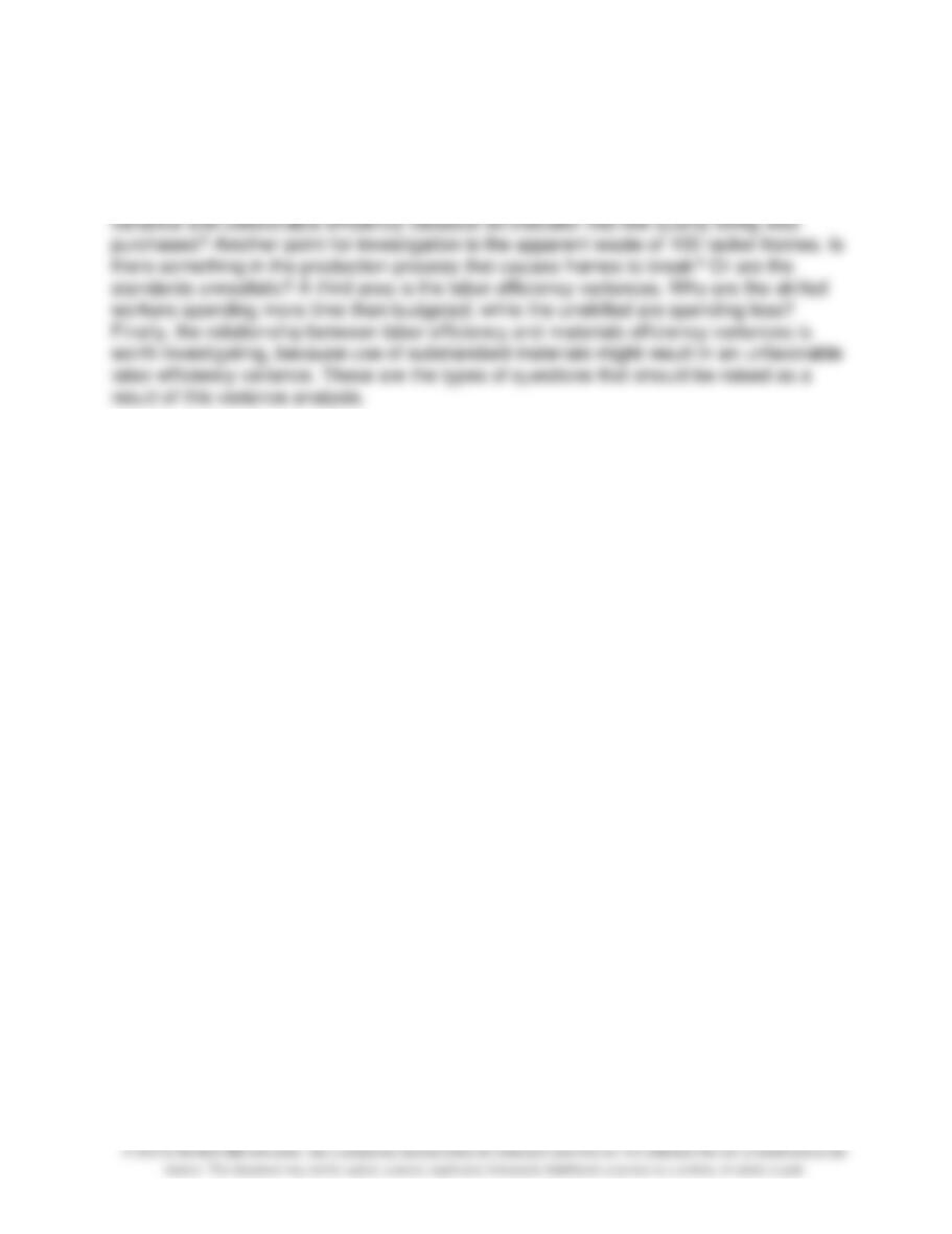
The variance breakdown in Exhibits A and B highlights the areas that Elmo and Otto
should research. One area involves the strings. Is the combination of a favorable price