Chapter 17 – Additional Topics in Variance Analysis
17-1
© 2014 by McGraw-Hill Education. This is proprietary material solely for authorized instructor use. Not authorized for sale or distribution in any
manner. This document may not be copied, scanned, duplicated, forwarded, distributed, or posted on a website, in whole or part.
Chapter 17
Additional Topics in Variance Analysis
Solutions to Review Questions
17–1.
False. Variances simply represent differences between plans and actual outcomes.
17–2.
Variances are usually “expensed” as a period cost (e.g., charged to Cost of Goods Sold).
Variances can also be prorated to accounts according to the standard cost balances in
17–3.
17–4.
Efficiencies can be realized for costs only. The sales activity variance captures the effect
on profit resulting from the difference between actual and budgeted sales.
17–5.
Chapter 17 – Additional Topics in Variance Analysis
17-2
17–6.
If a company has two or more products, a mix variance can arise even if the net effect of
all variances is zero. It might be very useful to learn about the mix variance because if the
17–7.
Examples include:
Steel mills which can process both new steel and recycled scrap
Chapter 17 – Additional Topics in Variance Analysis
17-3
Solutions to Critical Analysis and Discussion Questions
17–8.
By recognizing the materials price variance at the time of purchase, management
captures any difference between actual materials cost and the standard costs as reflected
17–9.
17–10.
In this situation the company is really selling just one product so a mix variance would not
be meaningful.
17–11.
In a hospital, as in other professional firms, billing rates vary with the level of the
professional person performing services. Hence, a physician’s time is billed at a higher
17–12.
Salary rates vary according to the classification of the service providers (e.g., nurses’ pay
is higher than nurse practitioners’ pay), and the hospital will budget a certain amount of
Chapter 17 – Additional Topics in Variance Analysis
17-4
17–13.
Disagree. The purpose of variance analysis is to identify items that are different from what
we expected (budgeted). Therefore, we should be as interested in favorable variances as
17–14.
Answers will vary. Variance analysis is helpful in any setting where budgets are
calculated, including business schools (and other academic institutions). In addition to the
Chapter 17 – Additional Topics in Variance Analysis
17-5
Solutions to Exercises
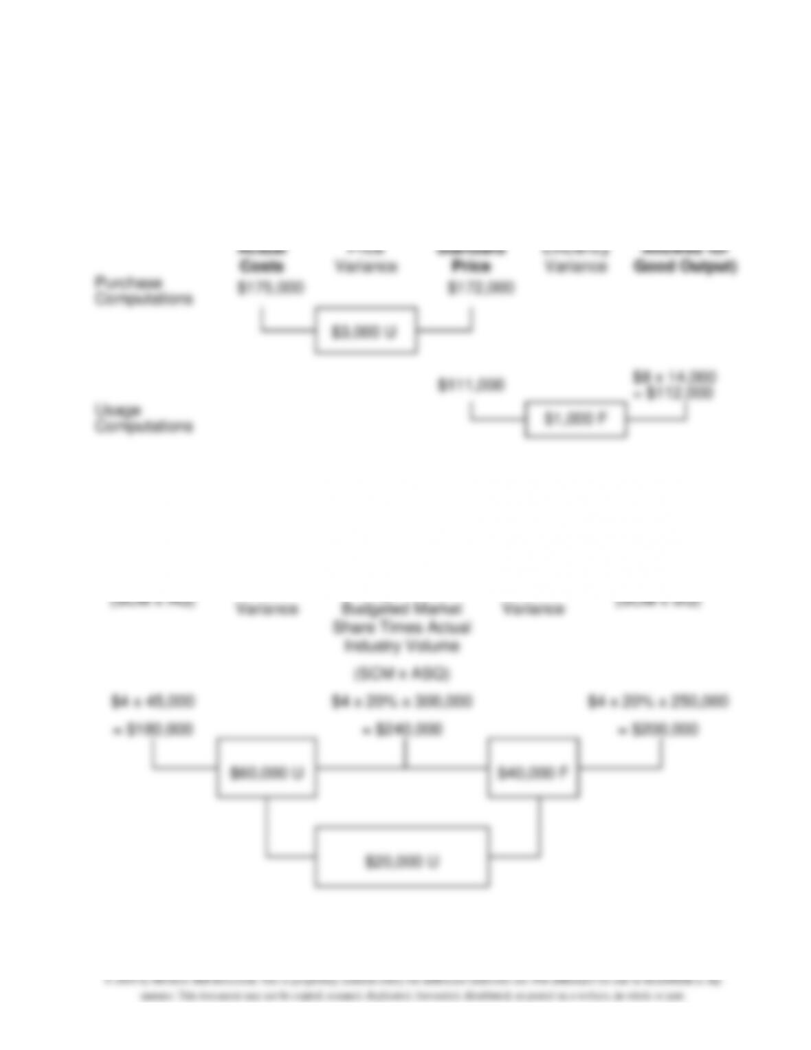
17–15. (15 min.) Variable Cost Variances: Materials Purchased And Used Are Not
Equal: Golden Company.
Actual
Costs
Price
Variance
Actual
Inputs at
Standard
Price
Efficiency
Variance
Flexible
Budget
(Standard
Allowed for
Good Output)
Purchase
Computations
$175,000
$172,000
$3,000 U
$111,000
$8 x 14,000
= $112,000
Usage
Computations
$1,000 F
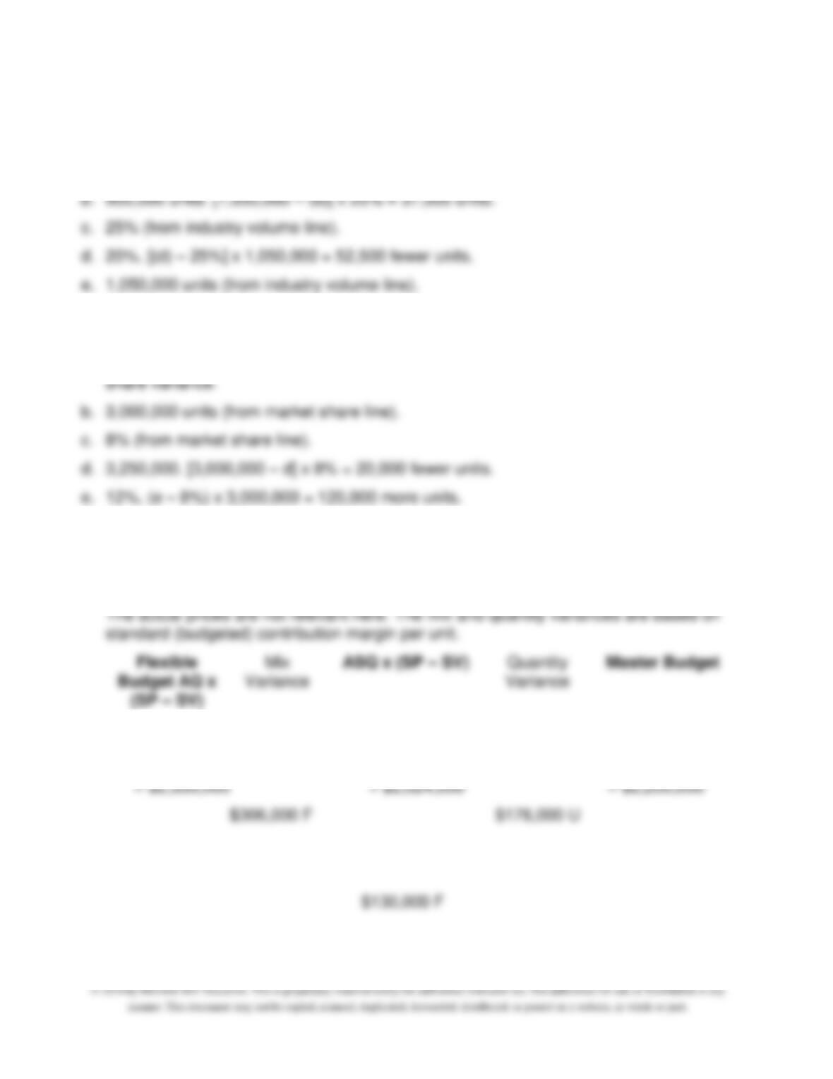
17–16. (15 min.) Industry Volume And Market Share Variances: Kay’s Auto
Products.
Flexible Budget
(SCM x AQ)
Market
Share
Variance
Standard Contribution
Margin Times
Budgeted Market
Share Times Actual
Industry Volume
(SCM x ASQ)
Industry
Volume
Variance
Master Budget
(SCM x SQ)
$4 x 45,000
= $180,000
$4 x 20% x 300,000
= $240,000
$4 x 20% x 250,000
= $200,000
$60,000 U
$40,000 F
$20,000 U
Chapter 17 – Additional Topics in Variance Analysis
17–17. (20 min.) Industry Volume And Market Share Variances—Missing Data.
a. 15,000 fewer units = 52,500 fewer units – 37,500 more units.
17–18. (20 min.) Industry Volume And Market Share—Missing Data.
a. 20,000 fewer units = 100,000 more units activity variance – 120,000 more units market
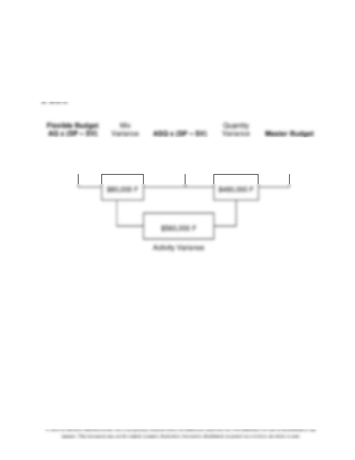
17–19. (20 min.) Sales Mix And Quantity Variances: AAA Electronics.
a. and b.
Chapter 17 – Additional Topics in Variance Analysis
Activity Variance
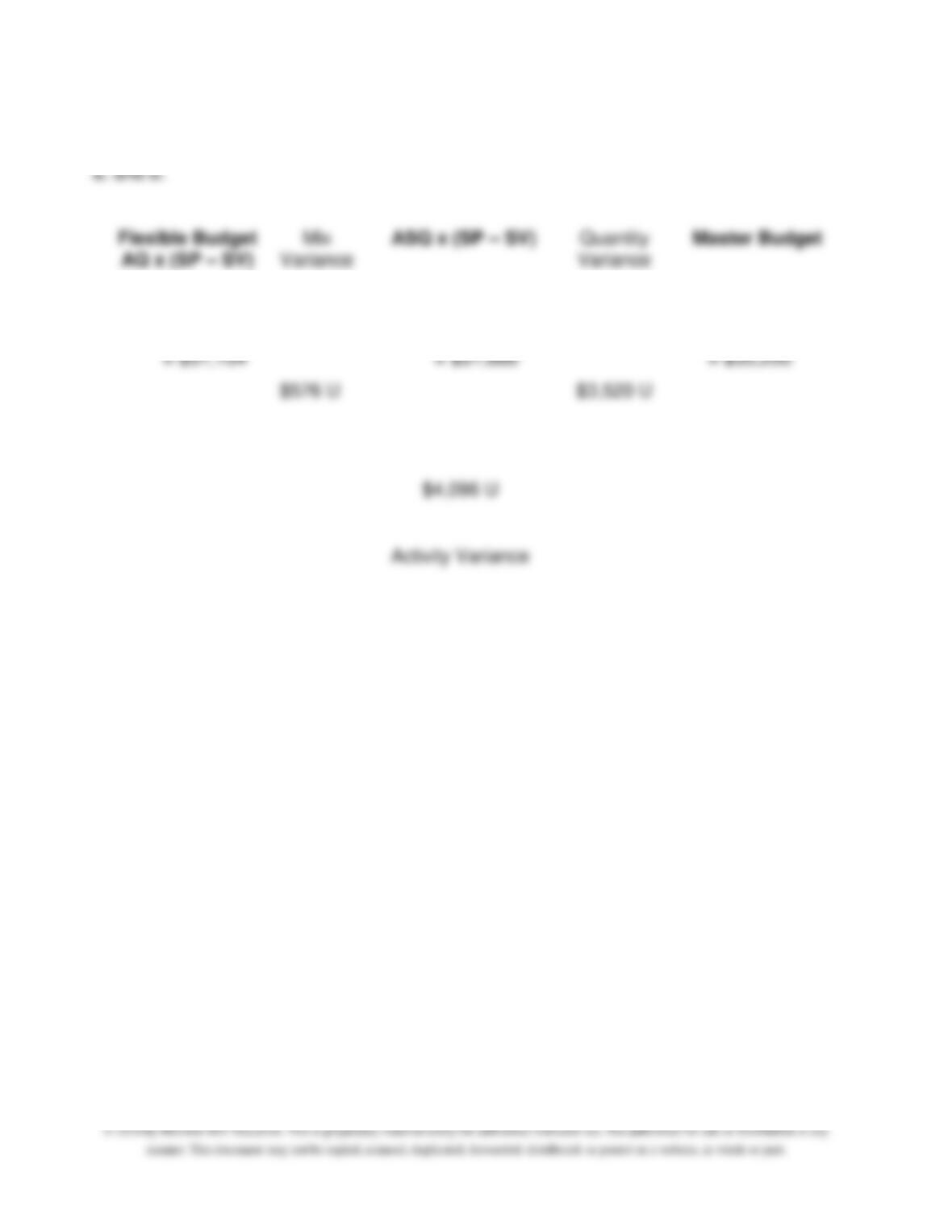
17–20. (20 min.) Sales Mix And Quantity Variances: Renee’s Rings.
Chapter 17 – Additional Topics in Variance Analysis
17–21. (20 min.) Sales Mix And Quantity Variances: Tapas By Tom.
Chapter 17 – Additional Topics in Variance Analysis
17-9
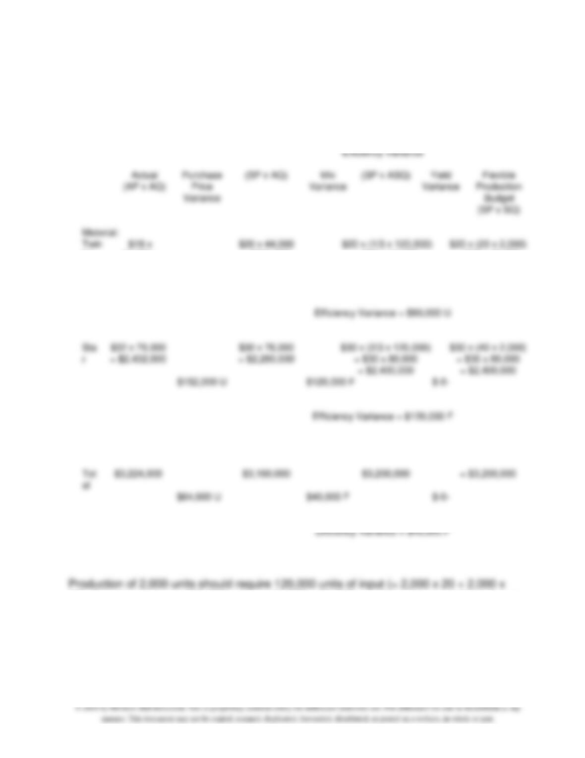
17–22. (35 min.) Materials Mix and Yield Variances: Huron Group.
a. and b.
Efficiency Variance
Actual
(AP x AQ)
Purchase
Price
Variance
(SP x AQ)
Mix
Variance
(SP x ASQ)
Yield
Variance
Flexible
Production
Budget
(SP x SQ)
Material:
Twin
kle
$18 x
44,000 =
$792,000
$20 x 44,000
= $880,000
$20 x (1/3 x 120,000)
= $20 x 40,000
= $800,000
$20 x (20 x 2,000)
= $20 x 40,000
= $800,000
$88,000 F
$80,000 U
$-0-
Efficiency Variance = $80,000 U
Sta
r
$32 x 76,000
= $2,432,000
$30 x 76,000
= $2,280,000
$30 x (2/3 x 120,000)
= $30 x 80,000
= $2,400,000
$30 x (40 x 2,000)
= $30 x 80,000
= $2,400,000
$152,000 U
$120,000 F
$-0-
Efficiency Variance = $120,000 F
Tot
al
$3,224,000
$3,160,000
$3,200,000
= $3,200,000
$64,000 U
$40,000 F
$-0-
Efficiency Variance = $40,000 F
Production of 2,000 units should require 120,000 units of input (= 2,000 x 20 + 2,000 x
40). Actual usage was 120,000 units (= 44,000 + 76,000), so there was no yield variance.
Chapter 17 – Additional Topics in Variance Analysis
17–10
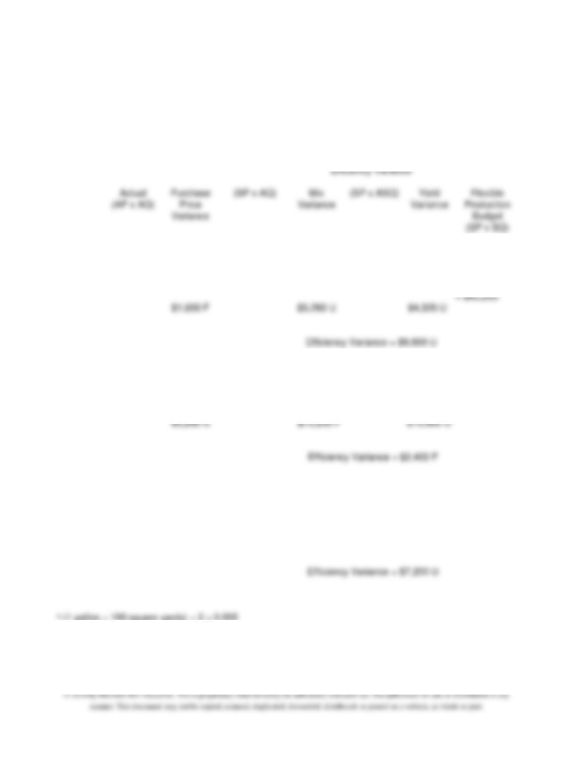
17–23. (35 min.) Materials Mix and Yield Variances: John’s Weed-B-Gone.
a. and b.
The actual purchase prices were $7.75 (= $51,150 ÷ 6,600) for Weed-X and $21.00 (=
$110,880 ÷ 5,280) for Pest-O.
Efficiency Variance
Actual
(AP x AQ)
Purchase
Price
Variance
(SP x AQ)
Mix
Variance
(SP x ASQ)
Yield
Variance
Flexible
Production
Budget
(SP x SQ)
Material:
Wee
d-X
$7.75 x
6,600
= $51,150
$8 x 6,600 =
$52,800
$8 x (1/2 x 11,880)
= $8 x 5,940
= $47,520
$8 x (0.005 a
x 1,080,000)
= $8 x 5,400
= $43,200
$1,650 F
$5,280 U
$4,320 U
Efficiency Variance = $9,600 U
Pes
t-O
$21 x 5,280
= $110,880
$20 x 5,280
= $105,600
$20 x (1/2 x 11,880)
= $20 x 5,940
= $118,800
$20 x (0.005 a
x 1,080,000)
= $20 x 5,400
= $108,000
$5,280 U
$13,200 F
$10,800 U
Efficiency Variance = $2,400 F
Tot
al
$162,030
$158,400
$166,320
= $151,200
$3,630 U
$7,920 F
$15,120 U
Efficiency Variance = $7,200 U