Chapter 16 – Fundamentals of Variance Analysis
16–50
16-59. (continued)
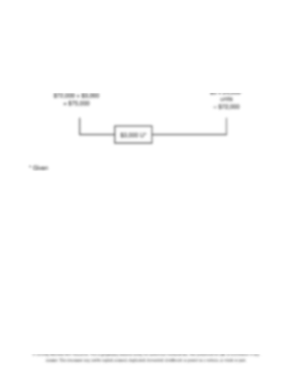
b. Overhead:
Actual
Costs
Applied
$72,000 + $3,000
= $75,000
$3 x 24,000*
units
= $72,000
$3,000 U*
* Given
Chapter 16 – Fundamentals of Variance Analysis
16–51
16–60. (40 min.) Variance Computations With Missing Data: Studio Company.
Note: The calculation of the fixed overhead budget amount makes this a challenging
problem. (Footnotes follow the calculations.)
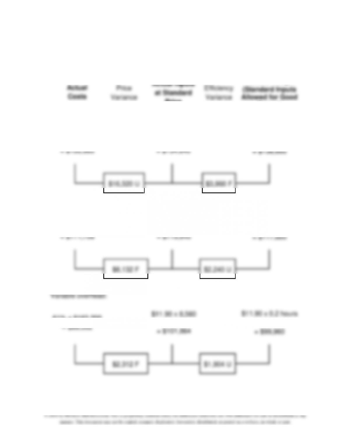
Direct materials:
Actual
Costs
Price
Variance
Actual Inputs
at Standard
Price
Efficiency
Variance
Flexible Budget
(Standard Inputs
Allowed for Good
Output)
(AP x AQ)
(SP x AQ)
(SP x SQ)
$1.85a x 81,600
gallons
= $150,960
$1.65 x 81,600
gallons
= $134,640
$1.65 x 2 gallons
x 42,000 units
= $138,600
$16,320 U
$3,960 F
Direct labor:
$13.05b x 8,560
hours
= $111,708
$14 x 8,560
hours
= $119,840
$14 x 0.2 hours
x 42,000 units
= $117,600
$8,132 F
$2,240 U
61% x $163,200
= $99,552
$11.90 x 8,560
hours
= $101,864
$11.90 x 0.2 hours
x 42,000 units
= $99,960
$2,312 F
$1,904 U
Chapter 16 – Fundamentals of Variance Analysis
16–60. (continued)
Chapter 16 – Fundamentals of Variance Analysis
16–53
16–61.
(50 min.) Comprehensive Variance Problem: Sweetwater Company.
Mountain Mist:
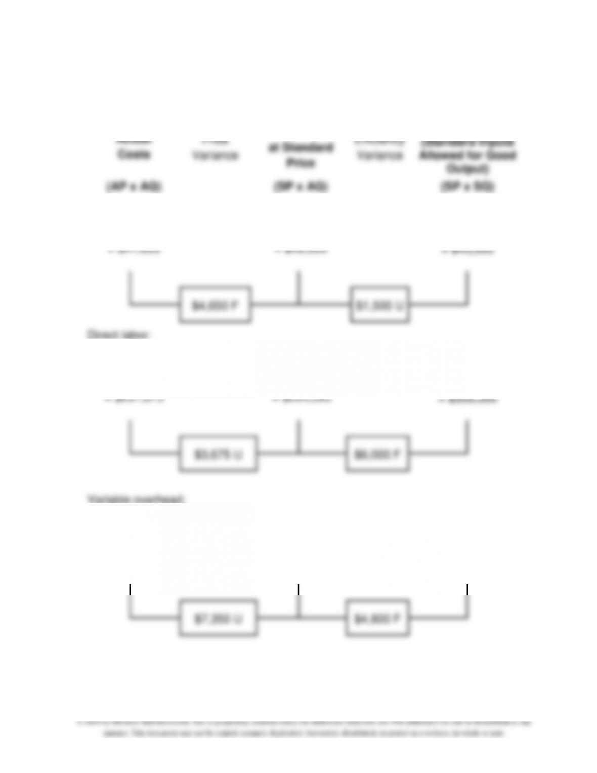
a. Direct materials:
Actual
Costs
Price
Variance
Actual Inputs
at Standard
Price
Efficiency
Variance
Flexible Budget
(Standard Inputs
Allowed for Good
Output)
(AP x AQ)
(SP x AQ)
(SP x SQ)
$13.50 x 3,100
ounces
= $41,850
$15 x 3,100
ounces
= $46,500
$15 x 3 ounces
x 1,000 units
= $45,000
$4,650 F
$1,500 U
Direct labor:
$60.75 x 4,900
hours
= $297,675
$60 x 4,900
hours
= $294,000
$60 x 5 hours
x 1,000 units
= $300,000
$3,675 U
$6,000 F
Variable overhead:
$242,550
$48 x 4,900
hours
= $235,200
$48 x 5 hours
x 1,000 units
= $240,000
$7,350 U
$4,800 F
Chapter 16 – Fundamentals of Variance Analysis
16–54
16–61. (continued)
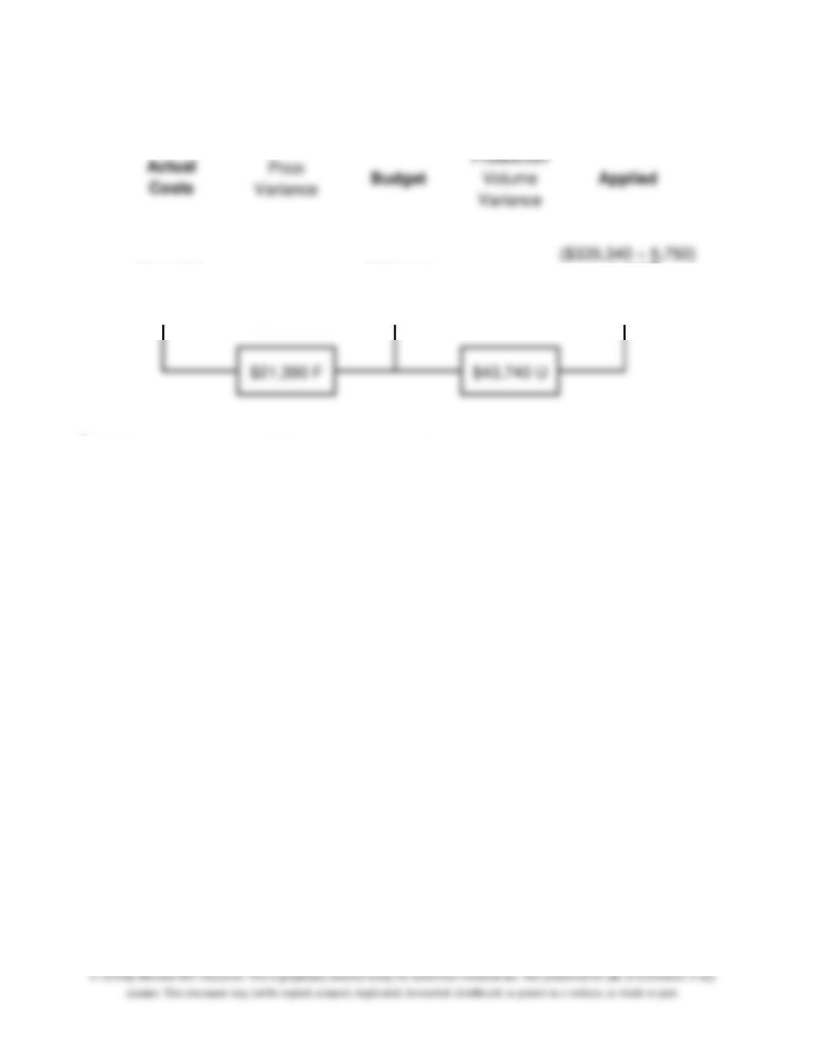
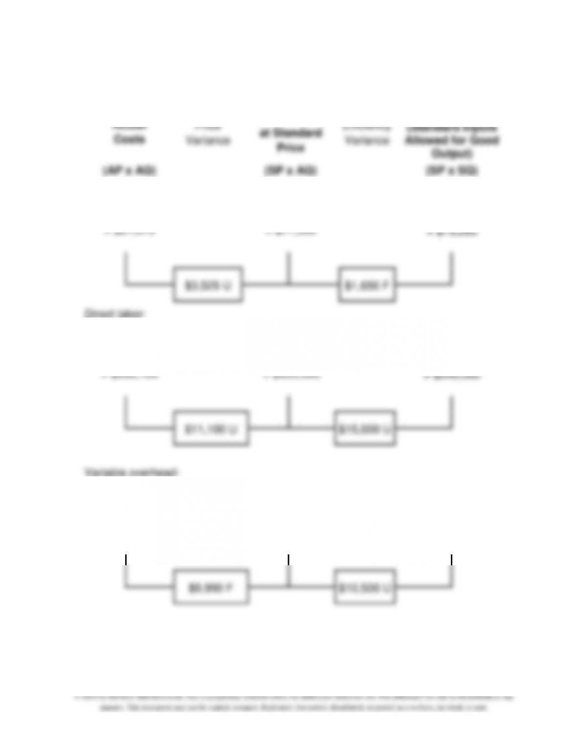
b. Fixed overhead:
Actual
Costs
Price
Variance
Budget
Production
Volume
Variance
Applied
$313,950
$335,340
($335,340 ÷ 5,750)
x 5,000a
= $291,600
$21,390 F
$43,740 U
a 5,000 hours allowed = 1,000 units produced x 5 hours per unit.
Chapter 16 – Fundamentals of Variance Analysis
16–55
16–61. (continued)
Valley Stream:
a. Direct materials:
Actual
Costs
Price
Variance
Actual Inputs
at Standard
Price
Efficiency
Variance
Flexible Budget
(Standard Inputs
Allowed for Good
Output)
(AP x AQ)
(SP x AQ)
(SP x SQ)
$17.25 x 4,700
ounces
= $81,075
$16.50 x 4,700
ounces
= $77,550
$16.50 x 4 ounces
x 1,200 units
= $79,200
$3,525 U
$1,650 F
Direct labor:
$76.50 x 7,400
hours
= $566,100
$75 x 7,400
hours
= $555,000
$75 x 6 hours
x 1,200 units
= $540,000
$11,100 U
$15,000 U
Variable overhead:
$378,510
$52.50 x 7,400
hours
= $388,500
$52.50 x 6 hours
x 1,200 units
= $378,000
$9,990 F
$10,500 U
Chapter 16 – Fundamentals of Variance Analysis
16–56
16–61. (continued)
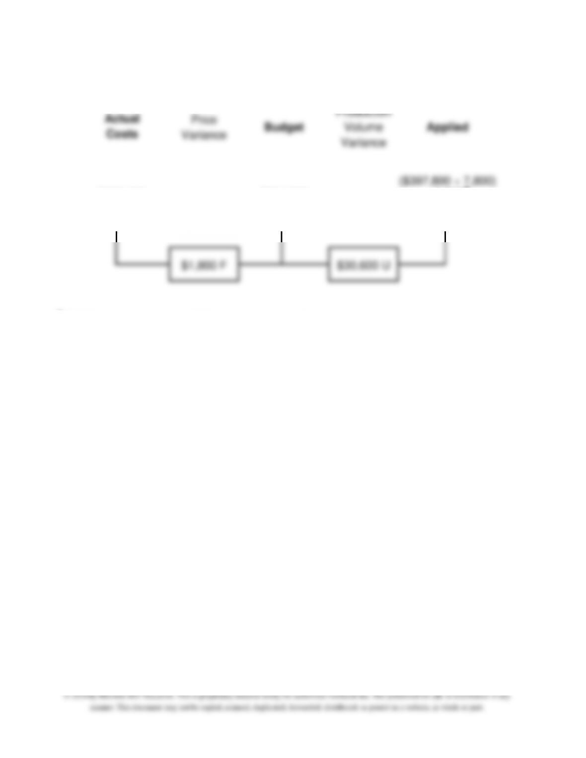
b. Fixed overhead:
Actual
Costs
Price
Variance
Budget
Production
Volume
Variance
Applied
$396,000
$397,800
($397,800 ÷ 7,800)
x 7,200a
= $367,200
$1,800 F
$30,600 U
a 7,200 hours allowed = 1,200 units produced x 6 hours per unit.
Chapter 16 – Fundamentals of Variance Analysis
16–57
Integrative Case
16–62. (60 min to 90 min) Performance Measurement and Variances: agm.com.
a.
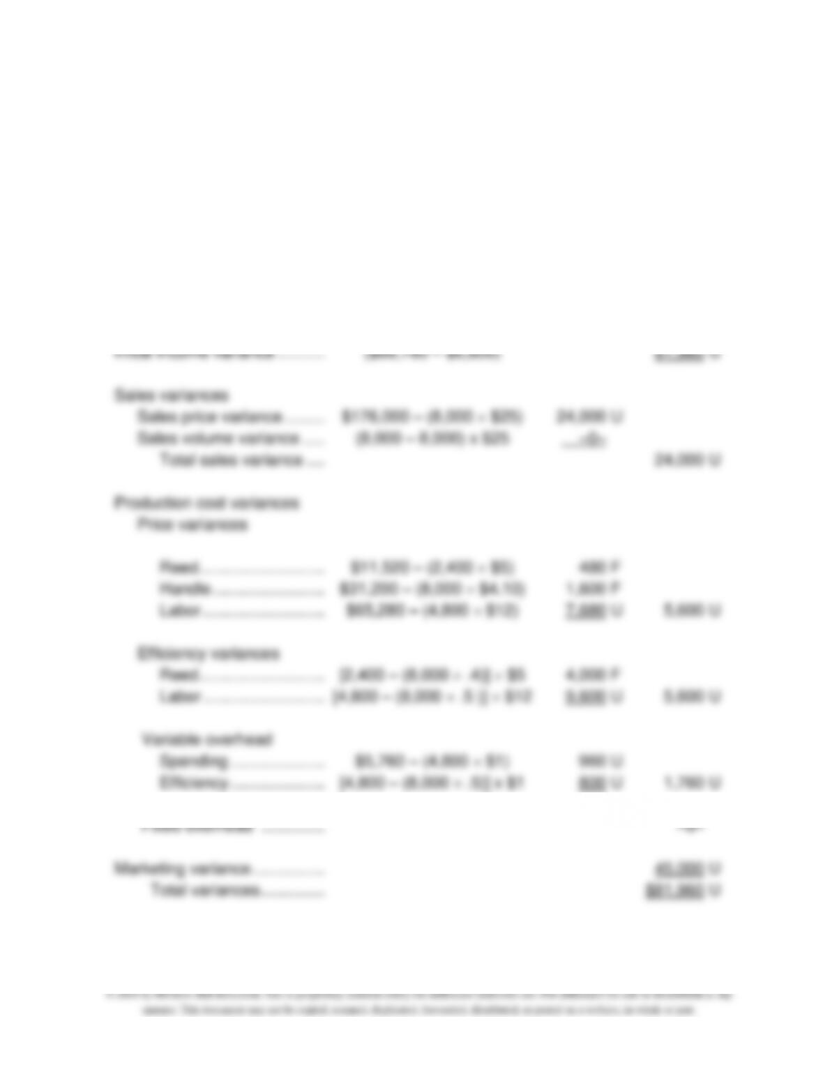
The following variances can be computed to understand better why actual income fell
short of budgeted income.
Factor:
Initial income variance …………………………..
($88,760 – $6,800)
81,960
U
Sales variances
Sales price variance ……….………………….
$176,000 – (8,000 $25)
24,000
U
Sales volume variance …………………………..
(8,000 – 8,000) x $25
–0–
Total sales variance …..………………………
24,000
U
Production cost variances
Price variances
Reed ………………………..…
$11,520 – (2,400 $5)
480
F
Handle ……………………..……
$31,200 – (8,000 $4.10)
1,600
F
Labor ……………………….….
$65,280 – (4,800 $12)
7,680
U
5,600
U
Efficiency variances
Reed ………………………..…
[2,400 – (8,000 .4)] $5
4,000
F
Labor ……………………….….
[4,800 – (8,000 .5 )] $12
9,600
U
5,600
U
Variable overhead
Spending ………………….……….
$5,760 – (4,800 $1)
960
U
Efficiency ………………….……….
[4,800 – (8,000 .5)] x $1
800
U
1,760
U
Fixed overhead …………………………..
–0–
Marketing variance ……………..……………
45,000
U
Total variances …………………………..
$81,960
U
Chapter 16 – Fundamentals of Variance Analysis
16–58
16-62. (continued)
b.
The two specific items in the case that deal directly with this are the material savings and
the strike. The estimated cost of the strike can be computed as:
Lost sales ………….……………….
400 baskets x $12.40 (budgeted contribution margin)
$ 4,960
Shipping …………………………..
13,000
Marketing ………….……………….
32,000
Total …………………………..
$49,960
We can think about including lost sales even though she sold the planned 8,000. She
might have been able to sell (and produce) more if there was no strike.
The materials savings of $8,000 (= 20% $5 8,000 units) are already incorporated in
the total material efficiency variance. There is no reason she should receive credit for
these and not be held responsible for the other efficiency losses.
c.
Certainly Mary is not responsible (in the sense of control) for the strike. However, she is
responsible for designing operations and selecting suppliers. Strikes are not unknown and
if she is not held accountable for the effect of strikes (or fires, or floods, etc.), she will not
include the possible costs in her decisions.
Should the contract be re-negotiated? This is a much more difficult question. There are (at
least) two factors that need to be considered here. First, since this is the first year of
operations, the budget against which Mary is evaluated is subject to a great deal of
uncertainty. That is, the benchmark might have been “wrong.” On the other hand, if the
contract is re-negotiated for this event, how effective can the budget be in the future?