5-46 (continued)
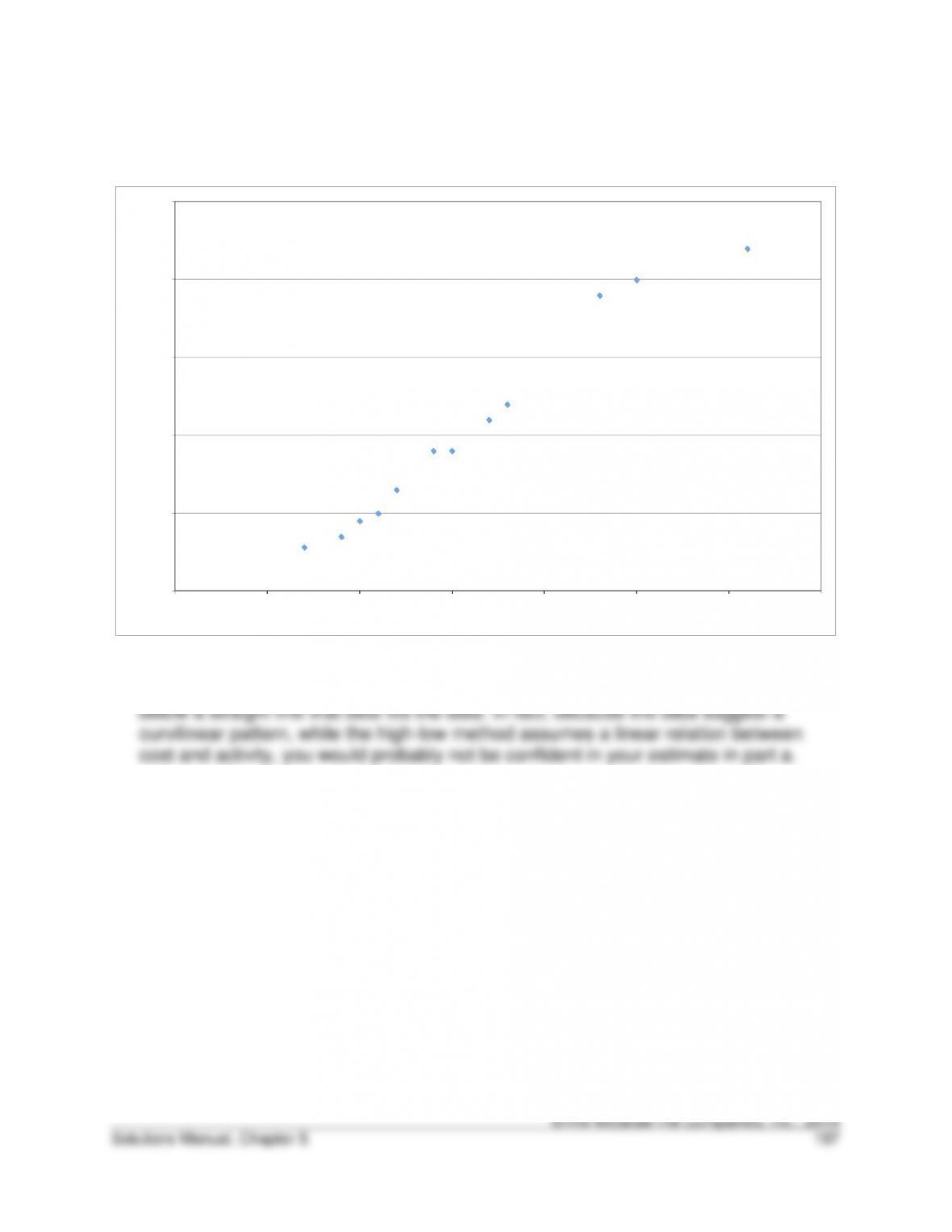
b. Scattergraph
$500
$550
$600
$650
$700
$750
30 35 40 45 50 55 60 65
Calls
Cost
c. The scattergraph shows a reasonably linear pattern, but the high point would lie
5-47. (30 min.) High-Low Method, Scattergraph: Academy Products.
a. High-low estimate
Machine
Hours
Overhead
Costs
Highest activity (month 5) …………………….
1,035,000
$3,700,000
Lowest activity (month 1) ……………………..
630,000
660,000
Variable cost =
Cost at highest activity – cost at lowest activity
Highest activity – lowest activity
5-47 (continued)
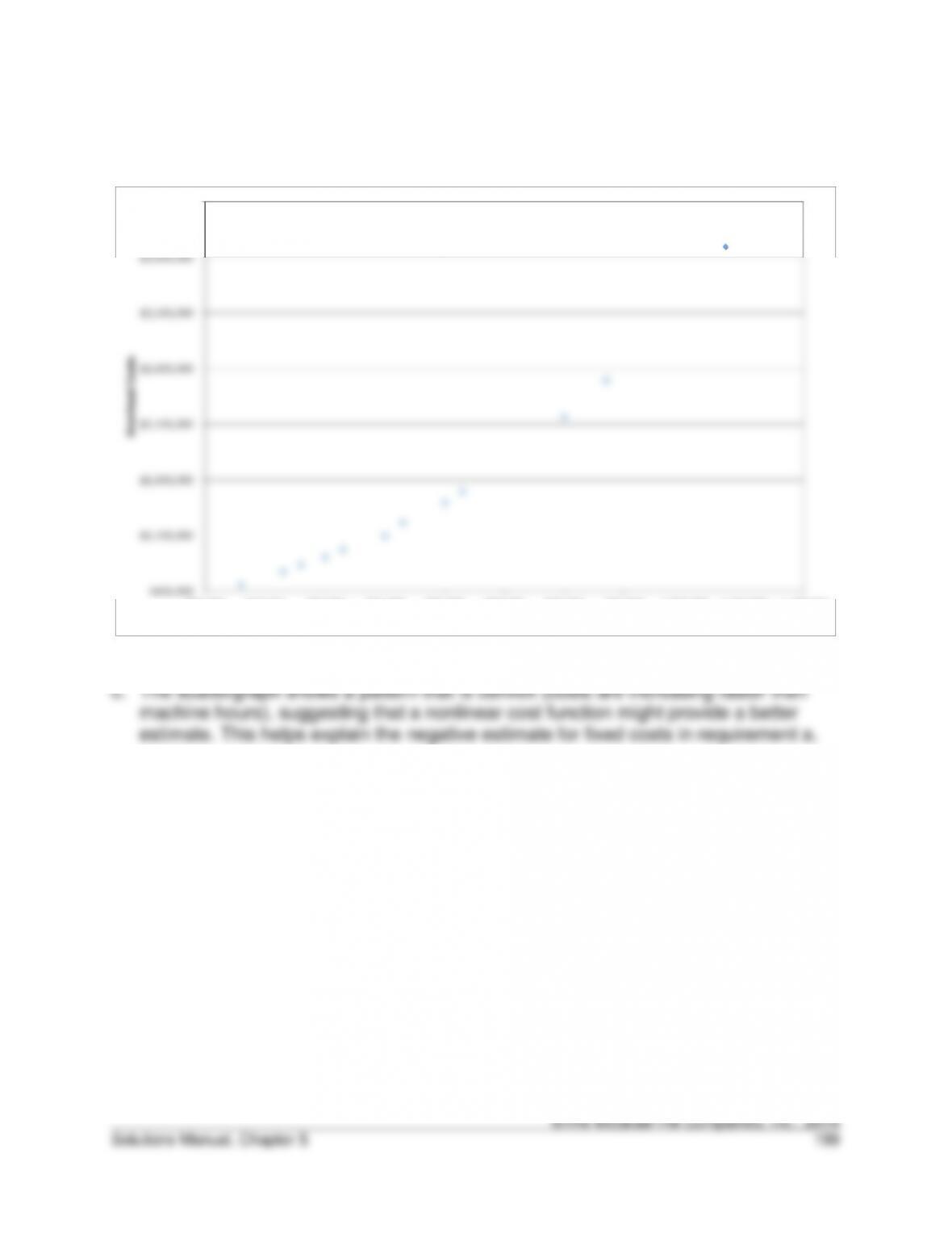
b. Scattergraph
$600,000
$1,100,000
$1,600,000
$2,100,000
$2,600,000
$3,100,000
$3,600,000
$4,100,000
600,000 650,000 700,000 750,000 800,000 850,000 900,000 950,000 1,000,000 1,050,000 1,100,000
Machine Hours
Overhead Costs
©The McGraw-Hill Companies, Inc., 2014
200 Fundamentals of Cost Accounting
5-48. (40 min.) Interpretation of Regression Results—Simple Regression Using a
Spreadsheet: Lucas Plant.
a. High-low estimate
Labor
Hours
Overhead
Costs
Highest activity (month 16) …………………..
395,938
$3,638,331
Lowest activity (month 11) ……………………
185,938
$2,314,436
Variable cost =
Cost at highest activity – cost at lowest activity
Highest activity – lowest activity
=
$3,638,331 – $2,314,436
395,938 – 185,938
= $6.30426 per labor-hour
Fixed
costs
=
Total costs – variable costs
=
$3,638,331 – $6.30426 x 395,938
=
$1,142,235
or
Fixed
costs
=
$2,314,436 – $6.30426 x 185,938
=
$1,142,235
The cost equation is:
Overhead costs = $1,142,235 + ($6.30426 per LH x Labor hours)
5-48. (continued)
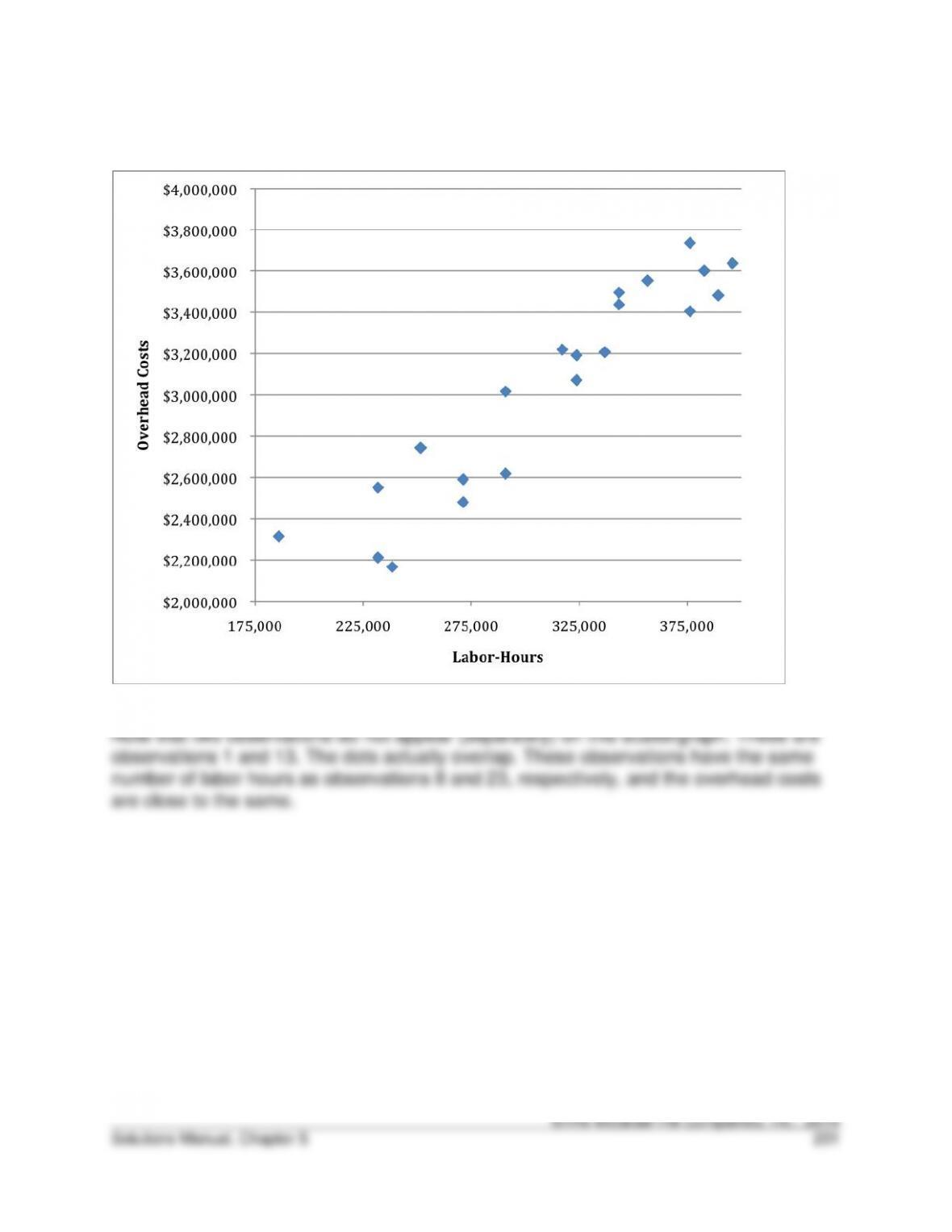
b. Scattergraph:
©The McGraw-Hill Companies, Inc., 2014
202 Fundamentals of Cost Accounting
5-48. (continued)
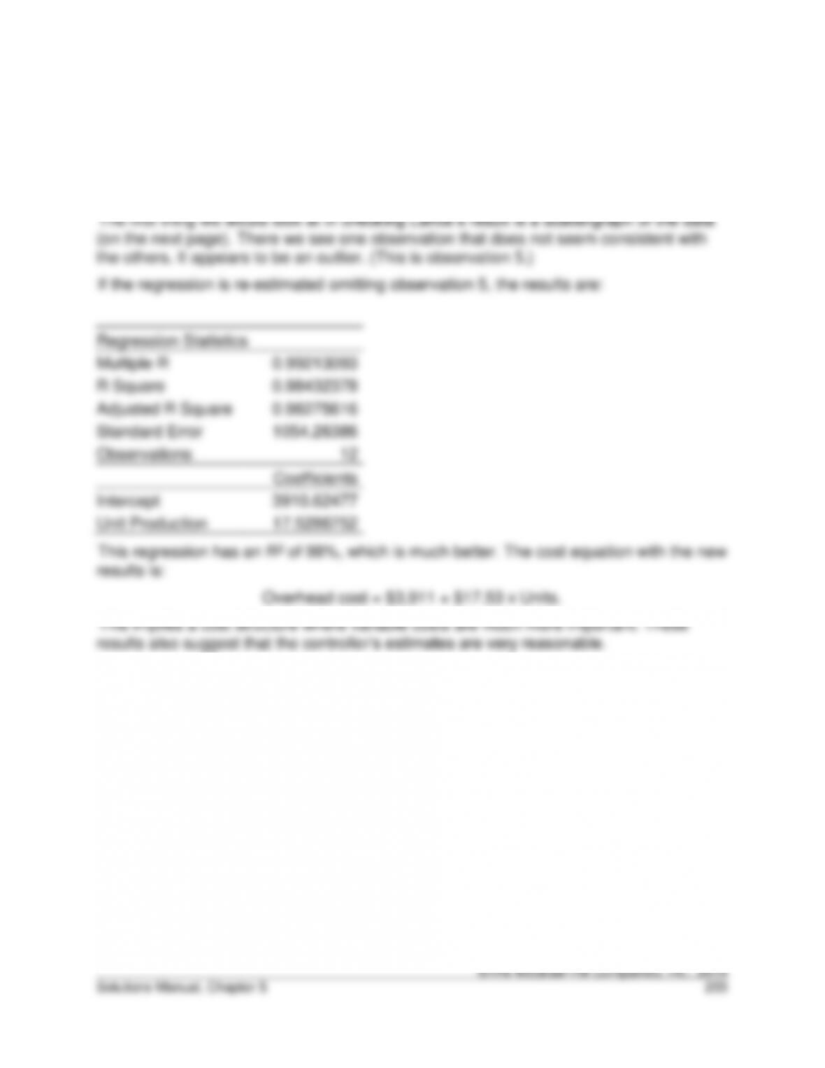
c. The results of the regression analysis are:
Regression Statistics
Multiple R
0.94877977
R Square
0.90018305
Adjusted R Square
0.89564591
Standard Error
176382.635
Observations
24
Coefficients
Intercept (Fixed costs)
$533,857.12
Labor Hours
$8.04
5-49. (30 min.) Interpretation of Regression Results—Simple Regression..
Although the correlation coefficient (or R) is 0.82, the R2, the percentage of the variation
in the independent variable “explained” by the dependent variable, is about 67%. This is
not low for “real,” data, but it is not as convincing as Lance would have us believe.
©The McGraw-Hill Companies, Inc., 2014
204 Fundamentals of Cost Accounting
5-49. (continued)
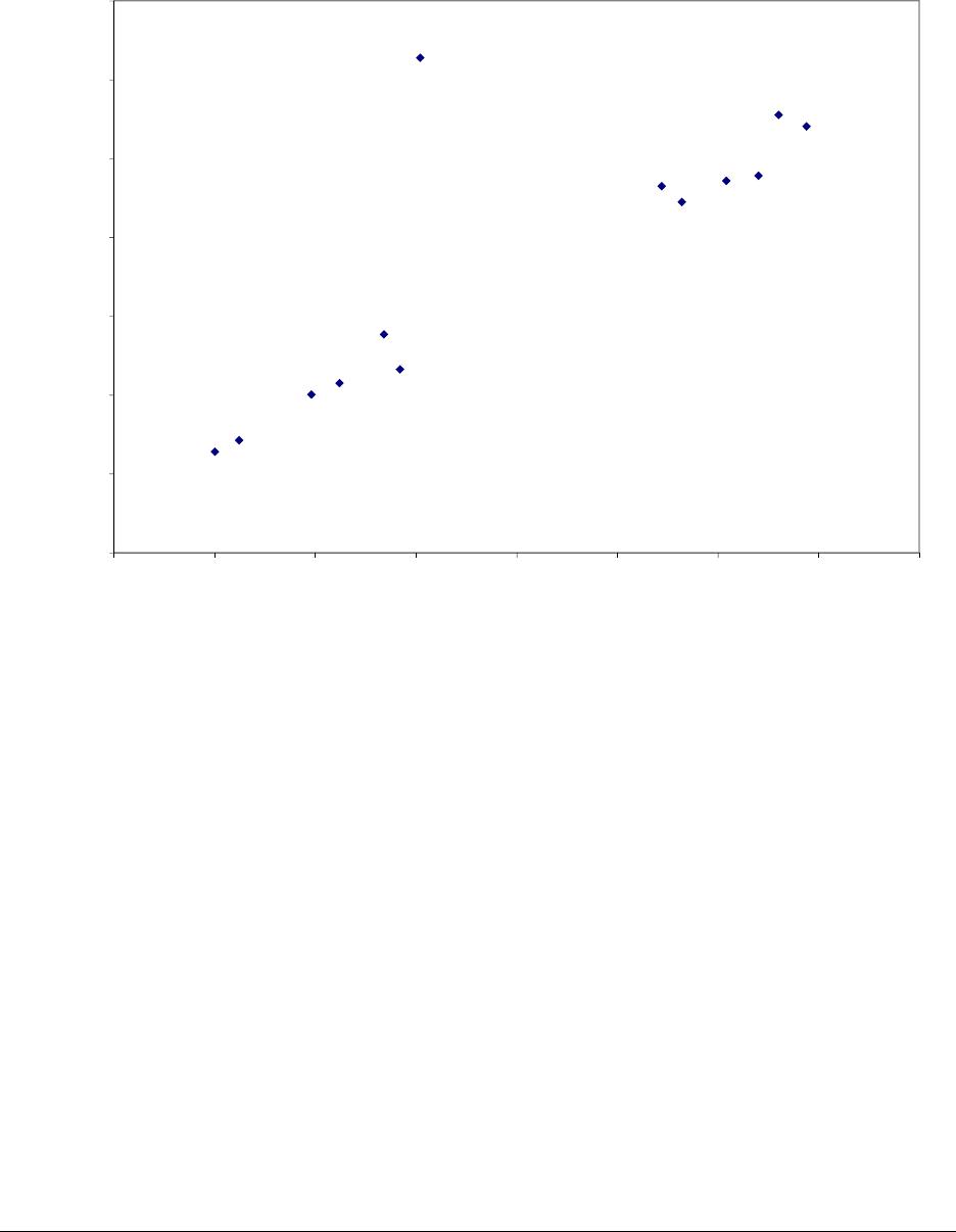
$50,000
$55,000
$60,000
$65,000
$70,000
$75,000
$80,000
$85,000
2800 3000 3200 3400 3600 3800 4000 4200 4400
Unit Production
Overhead Costs
5-50. (30 Min.) Interpretation of Regression Results—Multiple Choice: Eastern
College Business School.
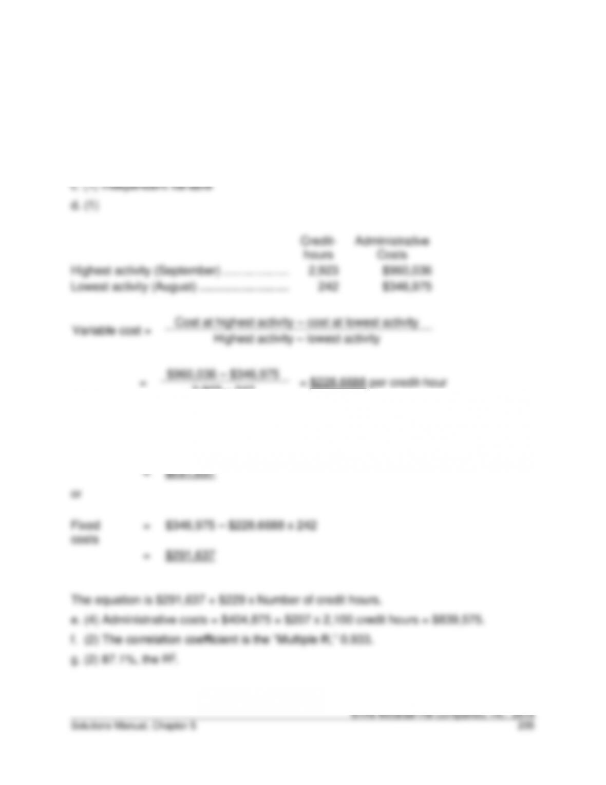
a. (5) Variable cost coefficient
b. (5) Dependent variable
Credit-
hours
Administrative
Costs
Highest activity (September) ………………..
2,923
$960,036
Lowest activity (August) ………………………
242
$346,975
Variable cost =
Cost at highest activity – cost at lowest activity
Highest activity – lowest activity
Fixed
=
Total costs – variable costs
=
$960,036 – $228.6688 x 2,923
Fixed
=
$346,975 – $228.6688 x 242
©The McGraw-Hill Companies, Inc., 2014
206 Fundamentals of Cost Accounting
5-51. (30 Min.) Interpretation of Regression Results: Simple Regression.
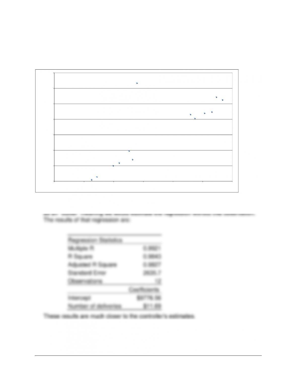
a. The first step in understanding the difference is to prepare a scattergraph of the
data:
140,000
150,000
160,000
170,000
180,000
190,000
200,000
210,000
10,000 11,000 12,000 13,000 14,000 15,000 16,000
Costs
Deliveries
Notice the one observation that appears to be unusual. (This is observation 5.)
Without knowing more about the reasons for the high cost, we might want to treat it