Chapter 04 -Fundamentals of Cost Analysis for Decision Making
4-41
4-57. (continued)
e. At an increase in the cost of labor from $16 to $19, the contribution margins per
constrained resource of labor (10,000 additional hours) would be as follows:
Contribution margins before labor cost increase:
Chapter 04 -Fundamentals of Cost Analysis for Decision Making
4-42
4-58. (20 min.) Optimum Product Mix: Bubble Company.
Bubble should produce only 1/2-litre bottles.
1/2-litre
1 -litre
Selling price …………………………
$ 15.00
$27.00
Variable costs
Materials …………………………...
4.00
7.00
Labor …………………………………
1.00
1.00
Total variable cost …………………
$ 5.00
$ 8.00
Contribution margin ……………….
$ 10.00
$ 19.00
÷ Hours to produce 1 unit ……….
÷ 1
÷ 2
Contribution margin per hour ….
$ 10.00
$9.50
An equivalent approach is to consider the machine depreciation when computing the
contribution margin (it is listed as variable with respect to hours). In the solution above,
we recognize that because we will operate the machine at capacity, the cost is really
fixed. If we treat it as variable, the solution is as follows:
1/2-litre
1 -litre
Selling price …………………………
$ 15.00
$27.00
Variable costs
Materials …………………………...
4.00
7.00
Labor …………………………………
1.00
1.00
Depreciation ………………………..
4,00
8.00
Total variable cost …………………
$ 9.00
$16.00
Contribution margin ……………….
$ 6.00
$11.00
÷ Hours to produce 1 unit ……….
÷ 1
÷ 2
Contribution margin per hour ….
$ 6.00
$5.50
Chapter 04 -Fundamentals of Cost Analysis for Decision Making
4-43
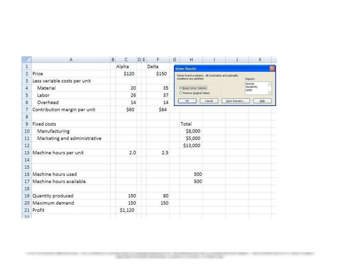
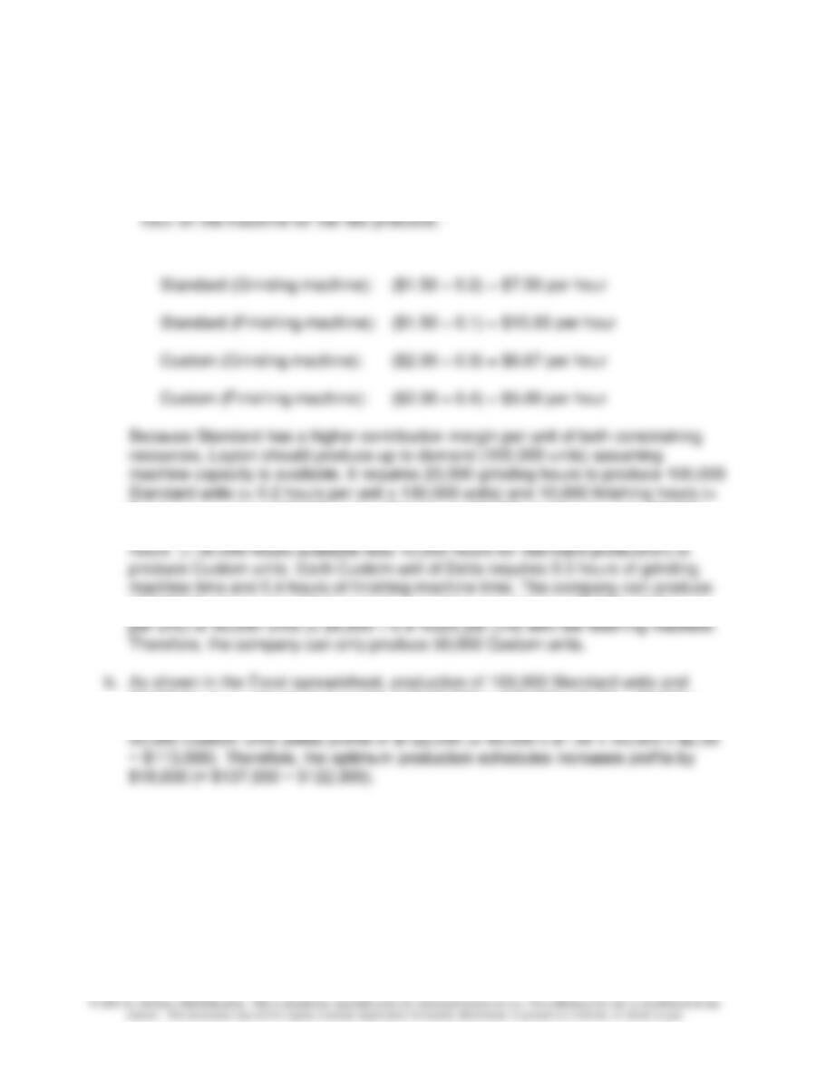
4-59. (20 min.) Optimum Product Mix – Excel Solver: Slavin Corporation.
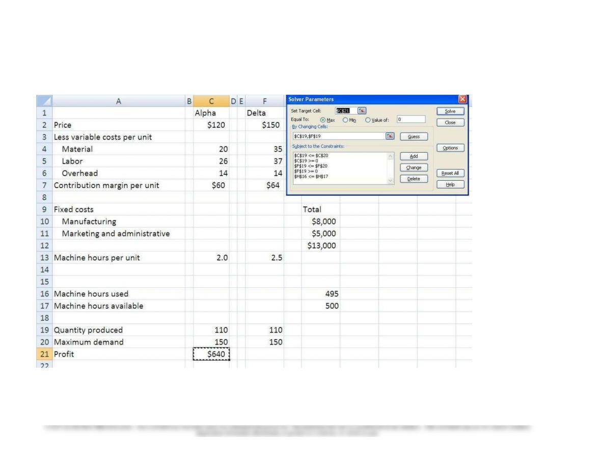
a. Slavin should produce 150 units of Alpha and 80 units of Delta. The next two pages
show the setup using Excel Solver and the solution. The problem can be solved
without Excel as follows. First, compute the contribution margins per hour on the
Chapter 04 -Fundamentals of Cost Analysis for Decision Making
4-44
4-59. (continued)
(i) Setup of Excel Solver:
Chapter 04 -Fundamentals of Cost Analysis for Decision Making
4-45
4-59. (continued)
(ii) Solution to problem:
Chapter 04 -Fundamentals of Cost Analysis for Decision Making
4-46
4-60. (20 min.) Optimum Product Mix – Excel Solver: Layton Machining
Company.
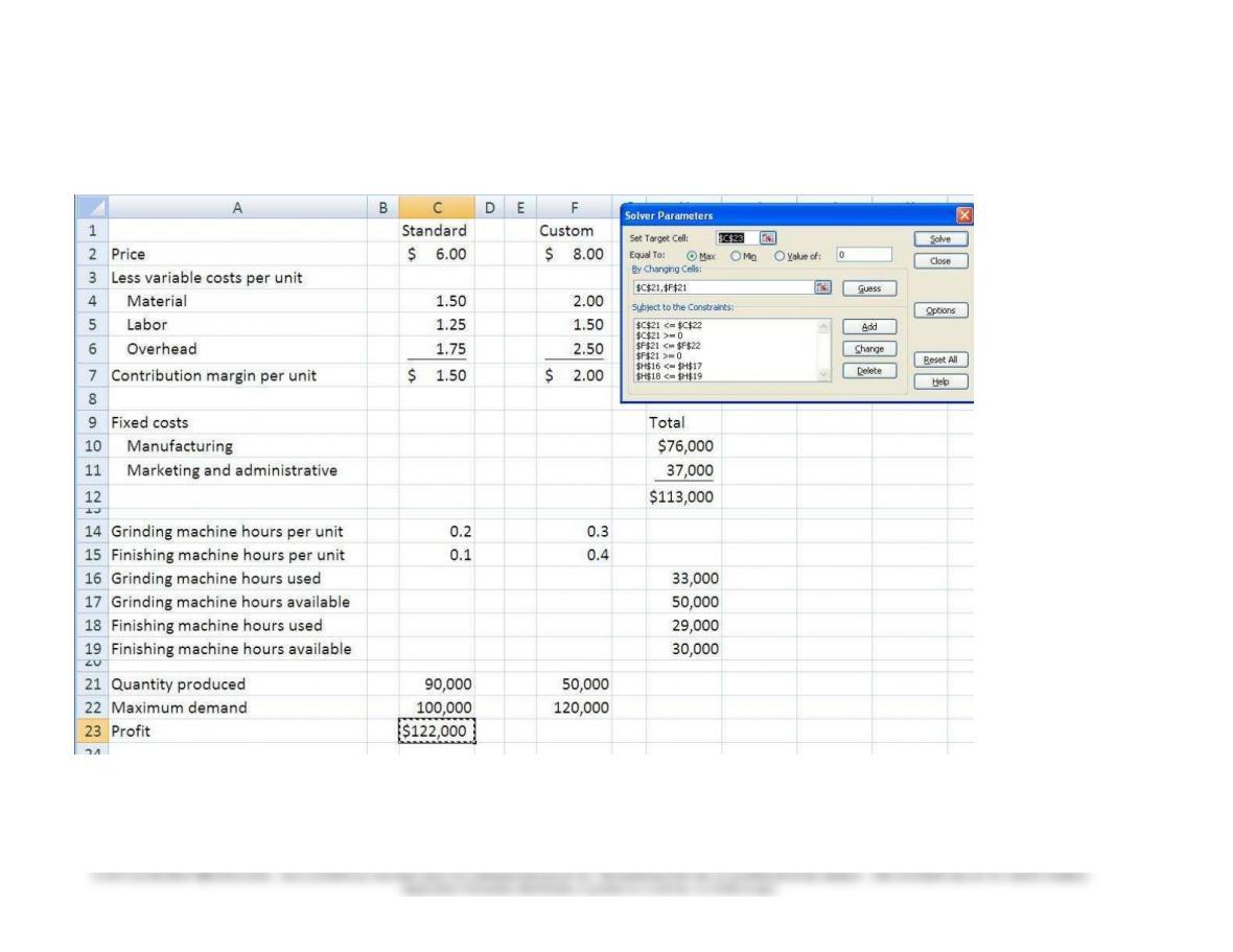
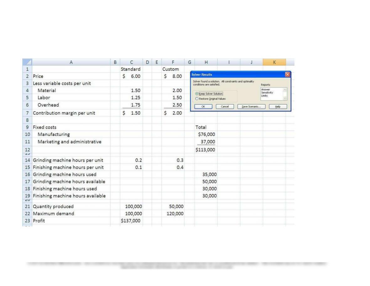
a. Layton should produce 100,000 Standard units 50,000 Custom units. The next
two pages show the setup using Excel Solver and the solution. The problem can
be solved without Excel as follows. First, compute the contribution margins per
0.1 hours per unit x 100,000 units). This leaves 30,000 grinding hours (= 50,000
hours available less 20,000 hours for Standard production) and 20,000 finishing
100,000 Custom units with the grinding machine constraint (= 30,000 ÷ 0.3 hours
50,000 Custom units leads to profits of $137,000 (= 100,000 x $1.50 + 50,000 x
$2.00 − $113,000). The current production schedule of 90,000 Standard units and
Chapter 04 -Fundamentals of Cost Analysis for Decision Making
4-47
4-60. (continued)
(i) Setup of Excel Solver:
Chapter 04 -Fundamentals of Cost Analysis for Decision Making
4-48
4-60. (continued)
(ii) Solution to problem:
Chapter 04 -Fundamentals of Cost Analysis for Decision Making
4-49
Solutions to Integrative Cases
4-61. (30 min.) The Effect of Cost Structure on Predatory Pricing: American
Airlines.
a The relation between variable cost and price is important in a predatory pricing case
because there is no rational economic reason for setting price below variable cost (and
Chapter 04 -Fundamentals of Cost Analysis for Decision Making
4-50
4-62. (120 min.) Make versus Buy: Liquid Chemical Company.
NOTE: Working this case requires knowledge of how to calculate discounted cash
flows.
a The four alternatives are:
• Alternative A: It is the “status quo,” i.e., Liquid Chemical Co. will continue making the
containers and performing maintenance.
the containers and provide the necessary maintenance.
b. The incremental cash flow analyses were conducted assuming a five-year time
horizon. Appendices I, II, III, and IV present the cash flow analyses for Alternatives A,
B, C, and D respectively, as well as more detailed information on the calculations.
General considerations for the incremental cash flows are provided below.
• Cash flows were not adjusted for inflation.
• 200 tons of GHL were purchased at the beginning of Year 0 (= $1,000,000/$5,000). 40
tons were consumed during Year 0 (expense of $200,000 = 40 tons X $5,000/ton),
leaving 160 tons in stock at the beginning of Year 1.
• Rent on the container department and the proportion of general administrative