
Chapter 05 – Cost Estimation
5-11
• In addition to the cost-estimating equation, the regression program provides other useful
statistics.
(1) Correlation coefficient (R, or multiple R) is a measure of the linear relation between
two or more variables, such as cost and some measure of activity. The closer R is to
±1.0, the closer the data points are to the regression line. Conversely, the closer R is
to zero, the poorer the fit of the regression line.
(2) Coefficient of determination (R2, or R-squared) is the square of the correlation
coefficient and interpreted as the proportion of the variation in the dependent variable
explained by the independent variable(s).
Example 1: From the regression results in Exhibit 5.3 where the linear relation between
overhead cost and repair-hours used is estimated,
Correlation coefficient (R) … .910
R2 …………………………... .828
Correlation coefficient (R) of .910 indicates that overhead cost and repair-hours are
moving nearly in tandem in the same direction. It is another way to say that the data
points are very close to the fitted regression line.
R2 of .828 means that nearly 83 percent of the changes in overhead costs can be
explained by changes in repair-hours. It is considered a good fit of the regression
equation to the data.
(3) t-statistic is the value of the estimated coefficient, b, divided by its standard error
(SEb). That is,
t =
The value of the estimated coefficient ( )
The standard error of ( )
b
b
b SE
.
• t-statistic is used to test whether the estimated coefficient on the independent variable is
significantly different from zero, indicating that the cost is not totally fixed. A t-statistic
greater than 2.0 is considered significant.
• The same conclusion on the significance level can be obtained from reading the p-value
from the regression result of a statistical package or a spreadsheet program. A very small
p-value indicates that the probability that the true value of the coefficient is zero, given
the data, is close to zero.

Chapter 05 – Cost Estimation
5-12
• A 95 percent confidence interval around b can be constructed by adding or subtracting
to b the appropriate t-value for the 95 percent confidence interval times the standard error
of b, or
b ± t × SEb.
That is, the variable cost coefficient should be between (b – t × SEb) and (b + t × SEb)
with a 95 percent probability.
Example 2: From the regression results in Exhibit 5.3 where the linear relation between
overhead cost and repair-hours used is estimated, b = $12.52 and SEb = 1.5843.
The value of t for a 95 percent confidence is available from probability tables to be t =
2.160. Therefore a 95 percent confidence interval for the coefficient b is
$12.52 ± 2.160 × 1.5843, or
between $9.10 and $15.94.
♦ The most commonly used regression technique is called ordinary least squares regression
(OLS).
• With this technique, the regression line is fitted so that the sum of the squares of the
vertical distances from each data point to the regression line is minimized.
• Organizations often exclude data for periods of unusual occurrences such as strikes,
extreme weather conditions, and shutdowns for equipment retooling in order to improve
the regression results. These extreme points are considered “outliers” that can
significantly affect the results.
• Scattergraphs plot data to reveal outliers that can be identified and omitted.
======================
Demonstration Problem 3
(Continued from Demonstration Problem 2)
John recently attended a workshop on statistical analysis. He was interested in applying the
regression analysis to solve the relation between overhead costs and machine hours.
Chapter 05 – Cost Estimation
5-13
Required:
1. Please help John determine the cost equation using the regression analysis and interpret
the regression results.
2. Predict overhead costs when 400 machine hours are expected to be spent for next month.
3. Indicate the t-statistic and the p-value associated with the estimated coefficient, b.
4. Given a t value of 2.228, construct the 95 percent confidence interval around the
estimated coefficient, b.
Solution:
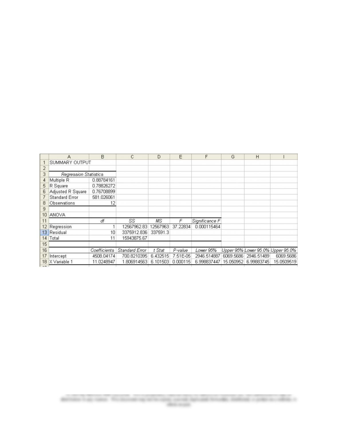
1. John’s analysis indicated that a logical relation exists between overhead costs and
machine hours. Microsoft Excel was used. Data on overhead costs were treated as Y, or
the dependent variable. Data on machine hours were treated as X, or the independent
variable. The regression results were displayed next.
The intercept represents the fixed costs, while X Variable 1 shows the variable cost per
unit of machine hour. The cost equation can be expressed as
Overhead costs = $4,508 per month + $11.02 × Number of machine hours used.
The correlation coefficient (Multiple R) of 0.888 points to a relatively good linear fit
between machines hours and overhead costs. The coefficient of determination (R square)
of 0.788 indicates that the machine hours as the cost driver managed to explain about
78.8% of variations in overhead costs, which is quite acceptable for accounting data.
2. For 400 machine hours to be spent next month, the overhead costs are expected to be
$4,508 per month + $11.02 × 400 machine hours = $8,916.

Chapter 05 – Cost Estimation
5-14
3. The t-statistic and the p-value are 6.1015 and 0.000115, respectively. The t-statistic is
considered significant (well above 2.0), as corroborated by a p-value that is close to zero.
4. The 95 percent confidence interval around the estimated coefficient, b, is
$11.02 ± 2.228 × 1.8069.
That means that, with a 95 percent confidence, the variable cost coefficient is between
$6.99 (= $11.02 – $4.03) and $15.05 (= $11.02 + $4.03).
======================
♦ Multiple regression, in which more than one predictor variables are used, may provide a better
estimate of the cost function.
• The cost equation can be modified as
TC = F + V1X1 + V2X2 + …,
where X1, X2, … represent different activities with the ability to explain the variations in
total costs and V1, V2, … the corresponding variable costs per unit.
• The adjusted R-squared (R2) is the correlation coefficient squared and adjusted for the
number of independent variables used to make the estimate. It is a better measure of the
association between X and Y than the unadjusted R2 value when more than one X
predictor is used.
• The t-statistic for each of the coefficients can also be tested for significance. That is, a
particular factor can be tested to see if it is indeed a cost driver.
• The additional data requirements for multiple regression models may limit their
usefulness in many applications.
LO 5-6 Identify potential problems with regression data.
♦ Some of the more common problems with using regression estimates include
(1) attempting to fit a linear equation to nonlinear data,
(2) failing to exclude outliers,
(3) including predictors with apparent, but spurious, relations to the dependent variables, and
(4) using data that do not fit the assumptions of regression analysis.

Chapter 05 – Cost Estimation
5-15
• When a firm is operating near its capacity limits, costs increase more rapidly than
activity. The linear cost estimate understates the slope of the cost line in the range close
to capacity, as shown in Exhibit 5.5.
• One way to overcome the nonlinearity problem is to use different regression equations
for different ranges of activity. Another approach is to model the nonlinearity explicitly,
but the resulting variable cost per unit won’t be constant.
• Observations that lie a significant distance from the regression line could have an
overwhelming effect on the regression estimates. Exhibit 5.6 shows such a case. The best
way to avoid this problem is to examine the data in advance (through scattergraph, for
example) and eliminate highly unusual observations before running the regression.
• Spurious relations may result from including many variables in the regression in the
hope of finding relations among the variables.
• Regression analysis relies on important assumptions, including
(1) the process for which costs are being estimated remains constant over time, and
(2) the errors in estimating the costs are independent of the cost drivers.
These assumptions are often violated in practice.
• A regression estimate is only an estimate. The users of regression should
(1) fully understand the method and its limitations,
(2) specify the model (i.e., the hypothesized relation between costs and cost predictors),
(3) know the characteristics of the data being used, and
(4) examine a plot of the data.
♦ Learning affects labor costs. The more experience that workers have in performing a task, the
less time they spend on it.
• Learning phenomenon is a systematic relationship between the amount of experience
in performing a task and the time required to perform it.
• Learning changes the process whose costs are being estimated, as shown in Exhibit 5.7.
Example 3: Using the incremental unit-time learning model with an 85 percent learning
rate for workers, whenever the output units are doubled (say from the first unit to the
second unit or from the second unit to the fourth unit, and so on), the time it takes to
produce the new output volume will be 85 percent of what it took to produce half of it
previously. That is,

Chapter 05 – Cost Estimation
5-16
Unit
Produced (X)
Labor time required to
produce the Xth unit
1
120 hours
2
102 (= 120 × .85)
4
86.7 (= 102 × .85)
8
73.695 (= 86.7 × .85)
…
…
Appendix B considers the mathematical foundation of learning and provides a way to
determine the labor time required to produce the 3rd, 5th, 6th, and 7th units, and so on.
• The learning phenomenon means that variable costs tend to decrease per unit as the
volume of activity increases. Most labor-related activities and costs are affected.
• Failing to recognize learning effects can have some unexpected consequences in
decision making and performance evaluation, among others.
LO 5-7 Evaluate the advantages and disadvantages of alternative cost
estimation methods.
♦ The most informative estimate of cost behavior results from using several methods because
each has the potential to provide information that the others do not.
• The more sophisticated method yields more accurate cost estimates than the simpler
methods do.
• All cost estimation methods make assumptions to simplify the analysis, including
(1) cost behavior with just one cost driver, and
(2) cost behavior being linear within the relevant range.
The reasonableness of the assumptions must be evaluated.
• Cost-benefit considerations dictate whether an approach is acceptable.
♦ No matter which method is used to estimate costs, the results are only as good as the data used.
• Using past costs and activity to predict future costs may be useful if a company’s
operations have followed a particular pattern in the past and the pattern is expected to
continue in the future.

Chapter 05 – Cost Estimation
5-17
• If the cost-activity relation changes, it should be necessary to adjust the estimated costs
accordingly or explicitly consider the change when developing the estimates. As the
number of adjustments increases, the resulting cost estimates tend to lose their objectivity.
• The usual data problems include
(1) missing data,
(2) outliers,
(3) allocated and discretionary costs,
(4) inflation, and
(5) mismatched time periods.
♦ Using several methods to arrive at a final estimate gives managers a likely range within which
actual costs will fall. Additional information may not be needed if the results converge, leading
to the same managerial decisions. Otherwise, more cost data have to be gathered.
LO 5-8 (Appendix A) Use Microsoft Excel to perform a regression analysis.
♦ The following steps are based on Version 12 of Excel (part of Microsoft Office 2007).
• Step 1: Ensure you have the Analysis TookPak installed.
• Step 2: Enter the data for the Dependent and Independent Variables.
• Step 3: Select Regression from the Data Analysis option.
• Step 4: Select the data to use in the regression.
• Step 5: Run the regression.
LO 5-9 (Appendix B) Understand the mathematical relationship describing
the learning phenomenon.
♦ The following mathematical relationship exists for the learning phenomenon:
b
Y aX
, where