
Chapter 05 – Cost Estimation
5-1
Chapter 5
Cost Estimation
Learning Objectives
1. Understand the reasons for estimating fixed and variable costs.
2. Estimate costs using engineering estimates.
3. Estimate costs using account analysis.
4. Estimate costs using statistical analysis.
5. Interpret the results of regression output.
6. Identify potential problems with regression data.
7. Evaluate the advantages and disadvantages of alternative cost estimation methods.
8. (Appendix A) Use Microsoft Excel to perform a regression analysis.
9. (Appendix B) Understand the mathematical relationship describing the learning
phenomenon.
Chapter Outline
I. WHY ESTIMATE COSTS?
II. BASIC COST BEHAVIOR PATTERNS
III. WHAT METHODS ARE USED TO ESTIMATE COST BEHAVIOR?
A. Engineering method
B. Account analysis method
C. Statistical cost estimation
1. Relevant range of activity
2. Scattergraphs and high-low estimates
3. Number of observations
4. High-low cost estimation
5. Statistical cost estimation using regression analysis
6. Obtaining regression estimates
7. Correlation coefficients
8. Confidence in the coefficients
D. Multiple regression
E. Practical implementation problems

Chapter 05 – Cost Estimation
5-2
1. Effect of nonlinear relations
2. Effect of outliers
3. Effect of spurious relations
4. Effects of using data that do not fit the assumptions of regression
analysis
5. Regression must be used with caution
F. Learning phenomenon
• Applications
IV. HOW IS AN ESTIMATION METHOD CHOSEN?
A. Data problems
B. Effect of different methods on cost estimates
V. SUMMARY
VI. APPENDIX A: REGRESSION ANALYSIS USING MICROSOFT EXCEL
♦ Using Microsoft Excel to estimate regression coefficients
VII. APPENDIX B: LEARNING CURVES
Key Concepts
LO 5-1 Understand the reasons for estimating fixed and variable costs.
♦ When managers make decisions, they need to compare the costs and benefits among alternative
actions. The costs associated with each alternative need to be estimated. The better these
estimates, the better the decisions managers will make.
♦ The most important characteristic of costs for decision making is how they behave. The study
of cost behavior deals with how costs vary with activity levels.
• Activities can be measured by volume, by complexity, or by any other cost driver.
• Volume refers to units of output, machine hours, pages typed, miles driven, etc.
• Complexity refers to the number of different products, the number of components in a
product, etc.
• Cost equation: TC = F + VX, where
TC = Total costs,
F = Fixed cost,
V = Variable cost per unit of activity, and
X = Volume of activity.
• Variable costs change proportionately with activity levels but fixed costs do not.
Chapter 05 – Cost Estimation
• Accounting systems accumulate costs by account, not by cost behavior. Therefore, only
total cost data are usually available, but not the breakdown of costs into fixed and
variable components.
• The In Action box points out the use of the engineering method to estimate the variable
cost of carrying text messages across the carriers’ network, which is close to zero.
♦ General methods to estimate the relation between cost behavior and activity levels include
(1) Engineering estimates,
(2) Account analysis, and
(3) Statistical methods (such as regression analysis).
• Different methods may likely lead to different results. More than one method should be
used so the results can be compared.
• In practice, operating managers often modify the estimates submitted by the controller’s
staff and apply their own best judgment as a final step in the estimation process.
• Both the strengths and weaknesses of these methods require attention.
LO 5-2 Estimate costs using engineering estimates.
♦ An engineering estimate is a cost estimate based on measurement and pricing of the work
involved in a task.
• To begin with, the size of the operation has to be determined, followed by a detailed
estimation of the necessary activities to carry out the operation and the costs associated
with each activity.
• In practice, labor time estimates come from a time and motion study. The time needed
for each step requiring labor will be multiplied by an estimated wage rate.

Chapter 05 – Cost Estimation
5-4
(1) It can detail each step required to perform an operation, making comparison possible
with similar operations in order to review productivity and to identify strengths and
weaknesses.
(2) It does not require data from prior activities in the organization, enabling estimation
of totally new activities.
(3) The company can identify where “slack” exists in the operations and adjust its plans
accordingly.
• Difficulties associated with engineering estimates:
(1) It can be expensive to use because it analyzes each activity involved in the business.
(2) Engineering estimates are often based on optimal conditions not reflected in actual
work. Inefficiencies and random events are usually ignored.
LO 5-3 Estimate costs using account analysis.
♦ Account analysis is a cost estimation method that calls for a review of each account making
up the total cost being analyzed.
• Account analysis is based on existing activities which may include the realities of
downtime, missed work, machine repair, and other factors that engineering estimates tend
to ignore in an ideal condition.
• The key step in account analysis is the identification of the relation between the activity
and the resulting cost – variable or fixed. The accountant’s judgment and experience are
critical.
• Exhibit 5.1 shows an example of cost estimation using account analysis. In this example,
each major class of overhead costs is itemized and divided into its estimated variable and
fixed components.
• Account analysis helps determine the fixed cost (F) and the variable cost per unit (V) in
the cost equation TC = F + VX. An estimate of the total cost (TC) in the future can be
made for other activity levels (X) as long as they are within the relevant range of the
operations.
• Management’s attention will be drawn to the variable cost amount as the cost that
changes with each change in volume.
• Account analysis relies heavily on the personal judgment which may not be entirely
objective as the decisions based on cost estimates often have major economic
consequences for the people making them.

Chapter 05 – Cost Estimation
5-5
• Account analysis usually uses prior period’s data alone which might include items that
were unusual, infrequent, and specific to that period that won’t be repeated in the future.
======================
Demonstration Problem 1
John, a cost analyst for a manufacturing firm, was asked to estimate the overhead costs at one of
the factories. He interviewed the supervisor and several workers there to get a feel of how
overhead costs changed. His experience with the cost accounting system pointed to the use of
machine hours as the cost driver for overhead items. Over the last 12 months, the total overhead
costs were $103,918, out of which John determined $4,620 to be fixed cost per month and the
rest variable cost. For the same period of time, 4,519 machine hours were incurred in that factory.
Required:
1. Please help John determine the general cost equation (TC = F + VX) that describes the
relation between overhead costs and machine hours in that factory.
2. If the factory expects to spend 400 machine hours next month, how much will the
overhead be?
Solution:
1. The variable cost component for the last 12 months had a total of $48,478 (= $103,918 –
$4,620 × 12), which can be divided by the machine hours involved to get the variable
overhead per machine hour. That is, V = $48,478 ÷ 4,519 machine hours = $10.73 per
machine hour. The cost equation can be stated as
Overhead costs = $4,620 per month + $10.73 × Number of machine hours used.
2. For 400 machine hours to be spent next month, the overhead costs are expected to be
$4,620 per month + $10.73 × 400 machine hours = $8,912.
======================
LO 5-4 Estimate costs using statistical analysis.
♦ When random and unusual events are present, statistical analysis can use data from the past
several periods of operations or several locations as the basis for estimating cost relations.
• Statistical theory allows for random events to be separated from the underlying relation
between costs and activities.
• Relevant range represents the limits within which a cost estimate may be valid.

Chapter 05 – Cost Estimation
5-6
• When past data are used, the relevant range for the projection is usually between the
upper and lower bounds of past activity levels for which data are available.
• Past data may be the only readily available, cost–effective basis for estimating costs. As
long as their limitations are recognized, past data can be a meaningful starting point.
• A scattergraph is a graph that plots costs against activity levels. This visual
representation of the data provides a quick indication of the fixed-variable relation of
costs and activities. It also indicates if the relation seems to change at certain activity
levels. Exhibit 5.2 shows the data and a scattergraph for a service center.
• The number of observations needed for scattergraph depends on the availability of the
data, the variability within the data, the relative costs and benefits of collecting reliable
data, and the length of time the current process has been in operation.
• A common rule of thumb is to use three years of monthly data if the physical processes
have not changed significantly within that time. If the operations have changed
significantly, data that predate the change may be misleading. Stable cost and activity
levels require a shorter time period (and fewer observations).
• A line can be visually fitted (by way of “eyeball judgment”) to the data points as closely
as possible and extended to the vertical axis on the scattergraph.
• The slope of the line represents the estimated variable cost per unit (i.e., the increase in
variable costs associated with an increase of one unit of activity), and the intercept with
the vertical axis represents an estimate of the fixed cost.
• When there are no observations of cost behavior around the zero activity level, the data
do not indicate the costs that would be incurred when the activity level was zero. In this
case, the interpretation of the intercept as the fixed cost will no longer be valid.
• An estimate on the basis of a scattergraph is subject to a high level of error, especially if
the points are scattered widely.
• Scattergraphs are usually used to illustrate the relations between costs and activity and
to point out any past data items that might be significantly out of line, but not the sole
basis for cost estimates.
♦ High-low cost estimation is a method to estimate costs based on two cost observations on the
scattergraph, usually at the highest and lowest activity levels.
• Activity can be defined in terms of units of production, hours of work, or any other
measure that makes sense for the problem at hand.
Chapter 05 – Cost Estimation
5-7
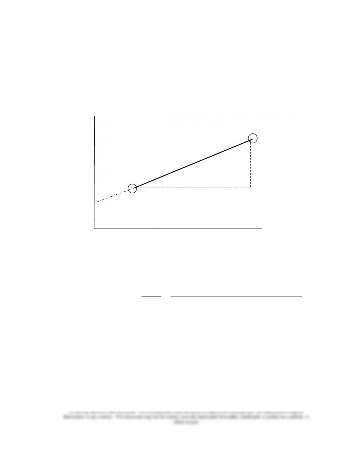
• The following illustration shows a scattergraph and a fitted line based on the highest
and lowest activity levels. The coordinates for the lowest point and the highest point are
(x1, y1) and (x2, y2), respectively. The cost equation to be estimated is TC = F + VX.
• The slope of the total cost line will be estimated first by using the following equation:
Variable cost per unit (V) =
y2 – y1
x2 – x1
=
Cost at highest activity – Cost at lowest activity
Highest activity – Lowest activity
.
• Once the slope of the total cost line is determined, the intercept can be estimated using
information from either the highest or the lowest activity level as both points belong to
the same fitted line.
Fixed cost (F)
= y2 – V ∙ x2
= Total cost at highest activity level – (Variable cost per unit × Highest activity level), or
Fixed cost (F)
= y1 – V ∙ x1
= Total cost at lowest activity level – (Variable cost per unit × Lowest activity level).
Total Cost (Y=TC)
Activity Level (X)
x
(x1, y1)
x
(x2, y2)
x
x
x
x
x
x
x
x
x
x
x
x

Chapter 05 – Cost Estimation
5-8
• Although the high-low method is easy to apply, use it carefully to ensure that the two
observations chosen to prepare the estimates represent cost and activity relations over the
range of activity for which the prediction will be made.
• When the scattergraph indicates that the highest and/or lowest points represent unusual
circumstances, other more representative highest and/or lowest point must be chosen
instead.
======================
Demonstration Problem 2
(Continued from Demonstration Problem 1)
The cost analyst, John, went back to the accounting information system to look for more relevant
data. The following breakdown of the overhead costs and the associated machine hours over the
same 12-month period was available:
Month
Overhead
Machine hours
1
$7,102
203
2
8,620
319
3
9,120
425
4
7,092
289
5
7,965
388
6
9,641
471
7
10,421
512
8
8,834
443
9
6,935
262
10
8,520
371
11
10,342
494
12
9,326
342
Total
$103,918
4,519
Required:
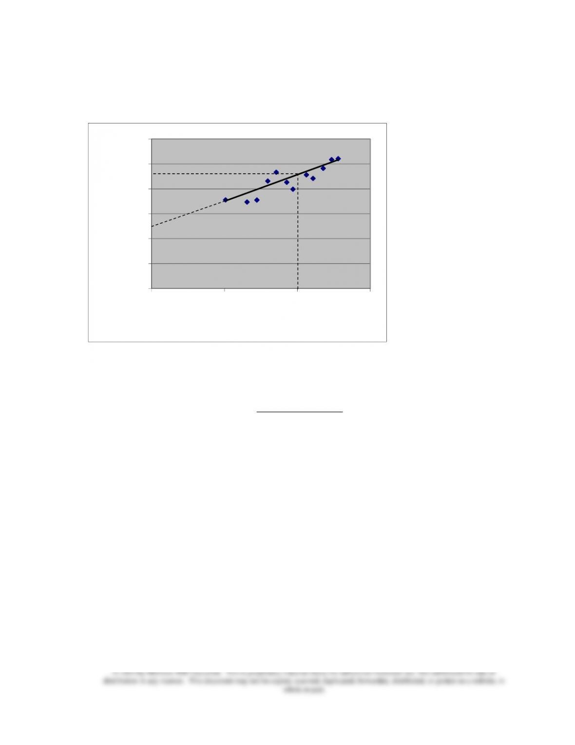
1. Plot the data using scattergraph.
2. Use the high-low method to estimate the cost function.
3. Predict overhead costs when 400 machine hours are expected to be spent for the coming
month.
Chapter 05 – Cost Estimation
5-9
Solution:
1.
0
2000
4000
6000
8000
10000
12000
0200 400 600
Overhead
Machine hours
2. The highest activity was 512 machine hours (MH) with overhead costs of $10,421; the
lowest activity was 203 machine hours (MH) with overhead costs of $7,102.
Variable cost per machine hour =
$10,421 – $7,102
512 MH – 203 MH
= $10.74 per machine hour.
Fixed cost = $10,421 – $10.74 × 512 machine hours = $4,922.
(Alternatively, Fixed cost = $7,102 – $10.74 × 203 machine hours = $4,922.)
The cost equation will be
Overhead costs = $4,922 per month + $10.74 × Number of machine hours used.
3. For 400 machine hours to be spent next month, the overhead costs are expected to be
$4,922 per month + $10.74 × 400 machine hours = $9,218.
======================

Chapter 05 – Cost Estimation
5-10
♦ Since the scattergraph and the high-low method can only offer rough approximation of the
relation between cost and activity, other cost estimation methods should also be considered,
especially those that rely on statistical approaches.
• Regression is a statistical procedure to determine the relation between variables. It is
designed to generate a line that best fits a set of data points.
• Since regression techniques use all the data points available, the resulting estimates
have a broader base than those based on a few select points.
• Additional information from regression allows managers to determine how well the
estimated regression equation describes the relations. Regression analysis also permits
the inclusion of more than one predictor, a helpful feature when more than one factor
affects costs.
• Many calculators and spreadsheet programs (such as Microsoft Excel®) can handle
regression analysis will little or no additional cost of using all available data points.
LO 5-5 Interpret the results of regression output.
♦ Independent variable is the X term, or predictor, on the right-hand side (RHS) of a regression
equation, while dependent variable is the Y term, or the left-hand side (LHS) of a regression
equation.
• The accountant or cost analyst is responsible for ensuring that the activities (i.e.,
independent variables) are logically related to costs to be estimated (i.e., dependent
variables).
• A simple regression uses just a single predictor.
• The intercept term from the output of a regression program (such as Exhibit 5.3) is an
estimate of fixed cost, though at zero activity it is usually outside the relevant range of
observations.
• The coefficient of the X term is an estimate of the variable cost per unit of activity,
which is usually labeled as b or given the variable name on the program output. This is
the slope of the cost line.
• The cost estimation equation based on the regression result is
Total cost = Intercept + (b × Activity level).