
Chapter 03 – Fundamentals of Cost-Volume-Profit Analysis
3-1
Chapter 3
Fundamentals of Cost-Volume-Profit Analysis
Learning Objectives
1. Use cost-volume-profit (CVP) analysis to analyze decisions.
2. Understand the effect of cost structure on decisions.
3. Use Microsoft Excel to perform CVP analysis.
4. Incorporate taxes, multiple products, and alternative cost structures into the CVP analysis.
5. Understand the assumptions and limitations of CVP analysis.
Chapter Outline
I. COST-VOLUME-PROFIT ANALYSIS
A. Profit equation
B. CVP example
1. Finding break-even and target volumes
2. Break-even volume in units
3. Break-even volume in sales dollars
4. Target volume in units
5. Target volume in sales dollars
C. Graphic presentation
D. Profit-volume model
E. Use of CVP to analyze the effect of different cost structures
F. Margin of safety
II. CVP ANALYSIS WITH SPREADSHEETS
III. EXTENSIONS OF THE CVP MODEL
A. Income taxes
B. Multiproduct CVP analysis
1. Fixed product mix
2. Weighted-average contribution margin
C. Alternative cost structures
IV. ASSUMPTIONS AND LIMITATIONS OF CVP ANALYSIS
V. SUMMARY

Chapter 03 – Fundamentals of Cost-Volume-Profit Analysis
3-2
Key Concepts
LO 3-1 Use cost-volume-profit (CVP) analysis to analyze decisions.
♦ Cost-volume-profit (CVP) analysis studies the relations among revenues, costs, and volume
and their effect on profit to help managers make decisions.
• Managers make decisions on volume, pricing, or incurring a cost that will impact profit.
• Profit equation: Operating profit (Profit) = Total revenues (TR) – Total costs (TC).
• Total revenues (TR) = Price (P) × Units of output produced and sold (X).
• Total costs (TC) = Variable cost per unit (V) × Units of output (X) + Fixed costs (F).
• The expanded version of the profit equation becomes
Profit = TR – TC
= PX – (VX + F)
= PX – VX – F
= (P – V)X – F, where
(P – V)X is the total contribution margin, the difference between total revenues (PX) and
total variable costs (VX). Contribution margin should be large enough to cover the fixed
costs and still provide for operating profit.
• Unit contribution margin = P – V.
• Alternatively, in CVP income statement format,
Total
Unit
Percentage
Sales revenue
PX
P
100%
– Variable costs
VX
V
V / P
= Contribution margin
(P – V)X
P – V
(P – V) / P
– Fixed costs
F
= Profit
(P – V)X – F
• In financial accounting, costs are classified as either manufacturing or administrative.
• In cost accounting, the concern is over cost behavior, where V represents the sum of
variable manufacturing cost per unit and variable marketing and administrative cost per
unit, and F the sum of total fixed manufacturing costs and fixed marketing and
administrative costs.

Chapter 03 – Fundamentals of Cost-Volume-Profit Analysis
3-3
• The operating profit can be derived
(1) algebraically from the profit equation, or
(2) from the company’s income statement.
Exhibit 3.1 demonstrates the process in a CVP income statement.
♦ CVP analysis helps answer the following questions:
(1) What volume is required to just break even (earning zero profit)?
(2) What volume is required to achieve a target profit?
• Break-even point is the volume level at which profits equal zero. That is,
Profit = 0 = (P – V)X – F.
• If the company makes many products, the volume is usually expressed in terms of sales
dollars; if only one product is available, units would be the measure of volume.
• Break-even volume in units (X*) =
Fixed cost (F)
Unit contribution margin (P- V)
.
• Contribution margin ratio =
Unit contribution margin (P-V)
Sales price per unit (P)
, the contribution margin
expressed as a percentage of sales revenue. Since
P-V
P
=
(P-V)X
PX
, the contribution
margin ratio remains the same at any level of activity.
• Break-even volume in sales dollars (PX*) =
Fixed cost (F)
PUnit Contribution margin (P V)
=
Fixed cost (F)
Contribution margin ratio ((P V)/ P)
.
• The volume to achieve a target profit may also be expressed either in units or in sales
dollars.
• Target volume in units (X**) =
Fixed cost (F) + Target profit
Unit contribution margin (P- V)
.
• Target volume in sales dollars (PX**) =
Fixed cost (F) Target profit
PUnit Contribution margin (P V)

Chapter 03 – Fundamentals of Cost-Volume-Profit Analysis
3-4
=
Fixed cost (F) + Target profit
Contribution margin ratio ((P V)/ P)
.
• Exhibit 3.2 provides a summary of target volume and break-even formulas.
♦ There are two ways to present the CVP relations graphically:
(1) CVP graph, and
(2) PV analysis.
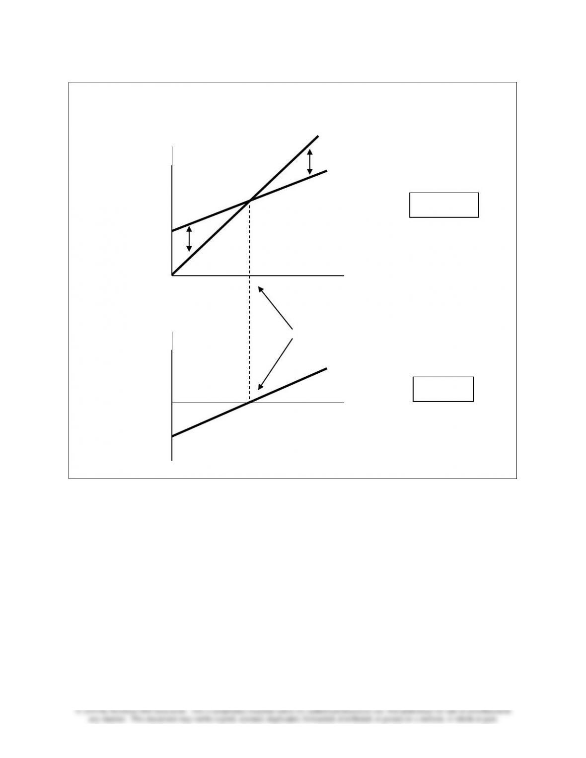
• CVP graph (Exhibit 3.3) plots total revenues against total costs at various activity levels
(volumes).
• The total revenue line (TR) starts at the origin (0, 0) with slope P, the price per unit. The
total cost line (TC) starts at intercept F with slope V, the variable cost per unit. The two
lines intersect at the break-even volume where TR = TC.
• Volumes lower than breakeven result in an operating loss (TR < TC); volumes higher
than breakeven result in an operating profit (TR > TC). The vertical distance between
TR and TC determines the amount of operating profit or loss.
• Profit-volume (PV) analysis is a version of the CVP analysis using a single profit line.
In Exhibit 3.4, the differences between TR and TC at various volumes are reduced to a
single profit line that starts at –F (the loss at zero volume, which equals fixed costs)
with slope the unit contribution margin. The vertical axis shows the amount of
operating profit or loss.
Chapter 03 – Fundamentals of Cost-Volume-Profit Analysis
3-5
Example 1: The relation between CVP graph and PV graph is presented below.
======================
Demonstration Problem 1
The Power Tool Division of ABC Hardware sells one product, Jig Saw, and has the following
data for the second quarter:
Units of output
1,200 units
Price per unit
$150
Variable cost per unit
90
Total fixed costs
48,000
Required: Determine
Volume
$
Volume
$
-F
F
0
TR = PX
TC = F + VX
Break-even volume
TR = TC
Operating profit
Operating loss
CVP graph
PV graph
TR – TC

Chapter 03 – Fundamentals of Cost-Volume-Profit Analysis
3-6
1. Quarterly operating profit when 1,200 units are sold.
2. Break-even volume in units and sales dollars.
3. Contribution margin ratio.
4. Sales dollars and units needed to generate an operating profit of $57,000.
5. Number of units sold that would produce an operating profit of 15% of sales dollars.
Solution:
1. Operating profit = (P – V)X – F = ($150 – $90) × 1,200 – $48,000 = $24,000.
2. Break-even volume in units (X*) =
V–P
F
=
90$150$
000,48$
= 800 units.
Break-even volume in sales dollars (PX*) = $150 × 800 units = $120,000.
3. Contribution margin ratio =
P
V–P
=
$150 $90
$150
× 100% = 40%.
4. Target profit = $57,000,
Sales dollars needed (PX**) =
F Target profit
(P-V)/P
=
%40
000,57$000,48$
= $262,500.
Units needed (X**) =
PX**
P
=
$262,500
$150
= 1,750 units.
5. Assume X to be the unknown number of units sold that would produce the operating
profit of 15% of sales dollars, then
(P – V)X – F = 15% × PX
($150 – $90)X – 15% × $150 × X = $48,000
X = 1,280 units.
======================
LO 3-2 Understand the effect of cost structure on decisions.
♦ Cost structure refers to the proportion of an organization’s fixed and variable costs to its total
costs.
• A firm (or an industry) with a high proportion of fixed costs, such as electric utilities, is
considered capital intensive; a firm (or an industry) with a high proportion of variable
costs, such as a grocery retailer, may be considered labor intensive.
• Operating leverage describes the extent to which an organization’s cost structure is
made up of fixed costs. It measures the sensitivity of a firm’s profit to changes in
volume.
Chapter 03 – Fundamentals of Cost-Volume-Profit Analysis
3-7
• A firm with a relatively high proportion of fixed costs, and therefore high operating
leverage, will experience a high break-even point and a high unit contribution margin.
For this type of firms, a small change in market demand will result in larger swing in
profits than firms with lower operating leverages.
• Firms with lower operating leverages are more flexible and better at withstanding
economic down times. On the other hand, during economic expansion, firms with higher
operating leverages will enjoy increased profit at a higher rate.
• Profit increase (decrease) as a result of improved (declining) sales can be calculated as
the product of operating leverage and sales increase (decrease) in percentage.
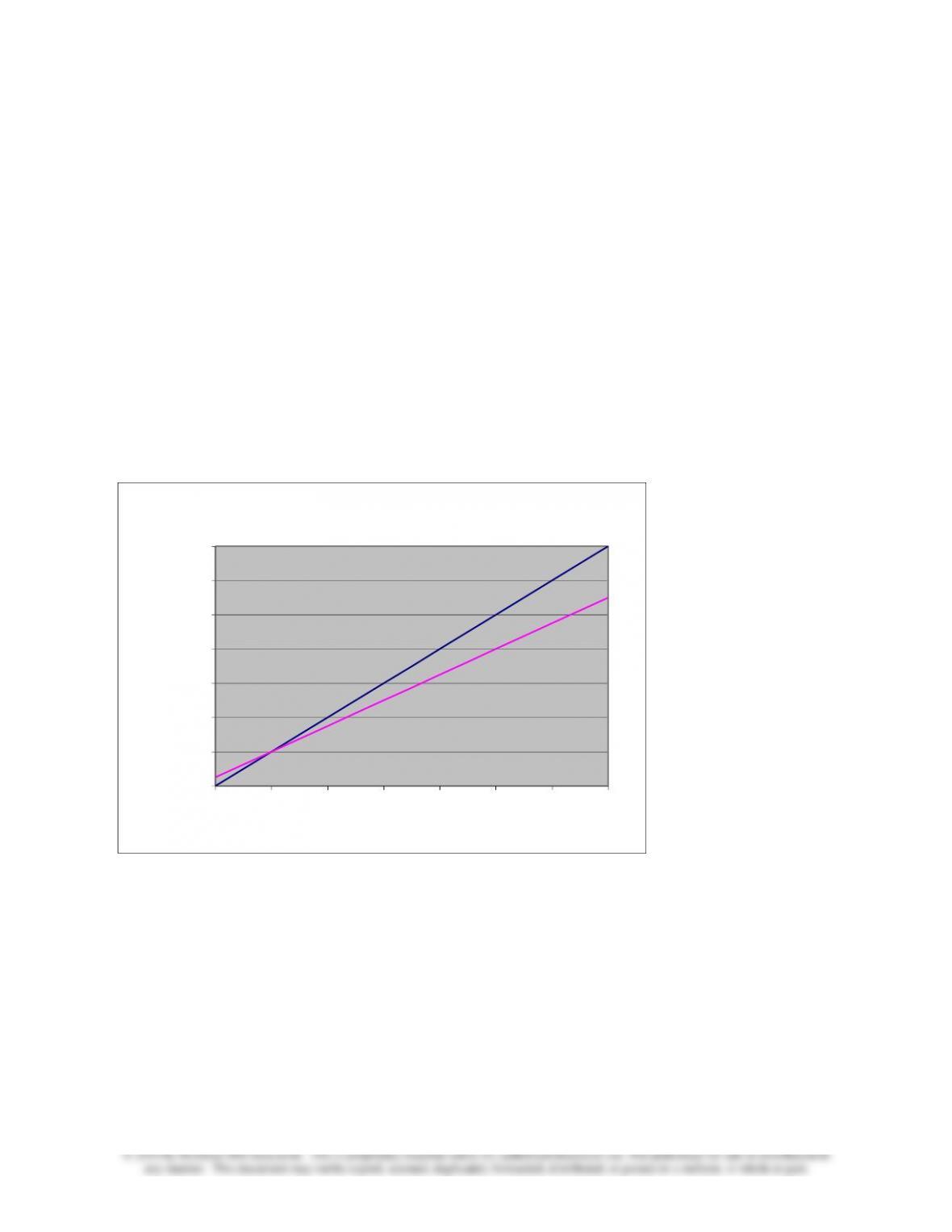
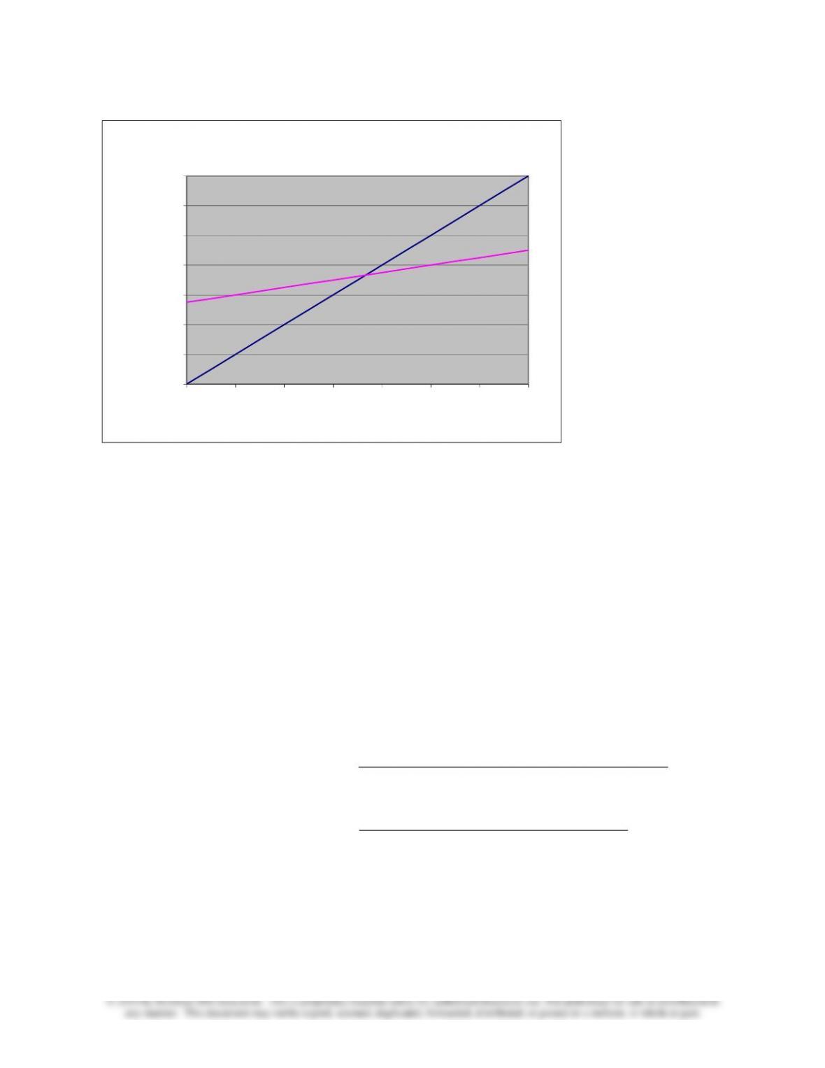
• Based on the data in Exhibit 3.5, the following two graphs illustrate the differences
between these two types of firms.
LO-LEV
0
200000
400000
600000
800000
1000000
1200000
1400000
0200000 400000 600000 800000 1000000 1200000 1400000
Units of output
$
TR
TC
Chapter 03 – Fundamentals of Cost-Volume-Profit Analysis
3-8
HI-LEV
0
200000
400000
600000
800000
1000000
1200000
1400000
0200000 400000 600000 800000 1000000 1200000 1400000
Units of output
$
• Different cost structures lead to different decisions that firms make concerning
operations and investments.
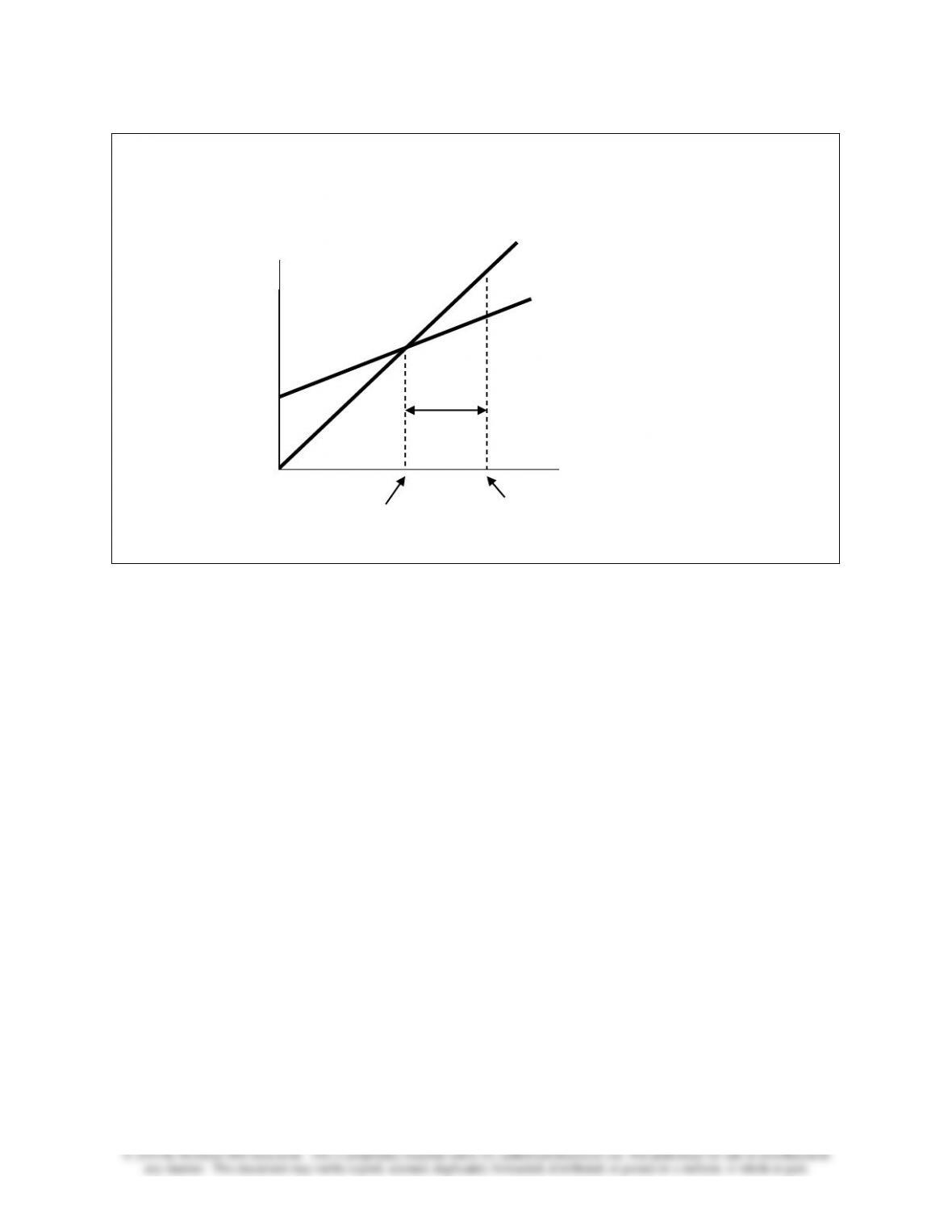
♦ Margin of safety refers to the excess of projected or actual sales over the break-even volume.
• Margin of safety (in units) = Sales volume – Break-even sales volume.
• The margin of safety indicates the risk of losing money that a company faces; that is,
the amount by which sales can fall before the company is in the loss area.
• In practice, the margin of safety also may be expressed in sales dollars or as a percent of
current or expected sales volume.
Margin of safety in sales dollars = Price per unit × Margin of safety in units.
Margin of safety percentage =
Margin of safety in sales dollars
Current or expected sales volume in sale dollars
× 100%
=
Margin of safety in units
Current or expected sales volume in units
× 100%.
TR
TC
Chapter 03 – Fundamentals of Cost-Volume-Profit Analysis
3-9
Example 2: Margin of safety is presented below.
LO 3-3 Use Microsoft Excel to perform CVP analysis.
♦ Spreadsheet programs such as Excel® will help analyze CVP relations. Analysis tools such as
Goal Seek can even accommodate alternative estimates of P, V, F, and target profits to conduct
so called “what–if” analyses. Exhibits 3.6 and 3.7 illustrate an example.
LO 3-4 Incorporate taxes, multiple products, and alternative cost structures
into the CVP analysis.
♦ In addition to the “what–if” analyses, more complications may be incorporated into the basic
CVP analysis to consider, for example, the fixed costs required to achieve a certain profit for a
given volume.
• Assuming t is the tax rate, then
After-tax profit = [(P – V)X – F] × (1 – t).
Volume
$
F
TR = PX
TC = F + VX
Break-even volume
Projected or
actual sales
Margin of
safety
(in units)