
Chapter 17 – Additional Topics in Variance Analysis
17–11
• A sales quantity variance occurs in multiproduct companies from the change in
volume of sales, independent of any change in sales mix.
Sales
quantity
variance
=
Standard contribution
margin per unit
×
(Quantity that would have been sold at the
standard mix – Budgeted sales quantity).
• The sales quantity variance measures the variance in sales quantity, holding the sales
mix constant.
• Although the variances can be calculated for each product sold to show the exact source,
the total variance is most frequently used for analysis.
• See Exhibit 17.5 for an example.
======================
Demonstration Problem 5
EZ Toys’ Stuffed Animals Division has two products: Bear and Monkey. Data on the two
products for October are as follows.
Bear
Monkey
Total
Standard selling price
$20
$12
Standard variable costs
12
8
Standard unit contribution margin
$8
$4
Budgeted sales quantity
2,500
7,500
10,000
Budgeted sales mix
25%
75%
Budgeted contribution margin
$20,000
$30,000
$50,000
Actual sales quantity
3,000
5,000
8,000
Actual sales mix
37.5%
62.5%
Budgeted contribution margin at actual quantities
$24,000a
$20,000
$44,000
Sales activity variance
$6,000 Ub
a $24,000 = $8 × 3,000 units.
b $6,000 U = $44,000 – $50,000.
Required:
Determine the Stuffed Animals Division’s sales mix and sales quantity variances for October.
Chapter 17 – Additional Topics in Variance Analysis
17–12
Solution:
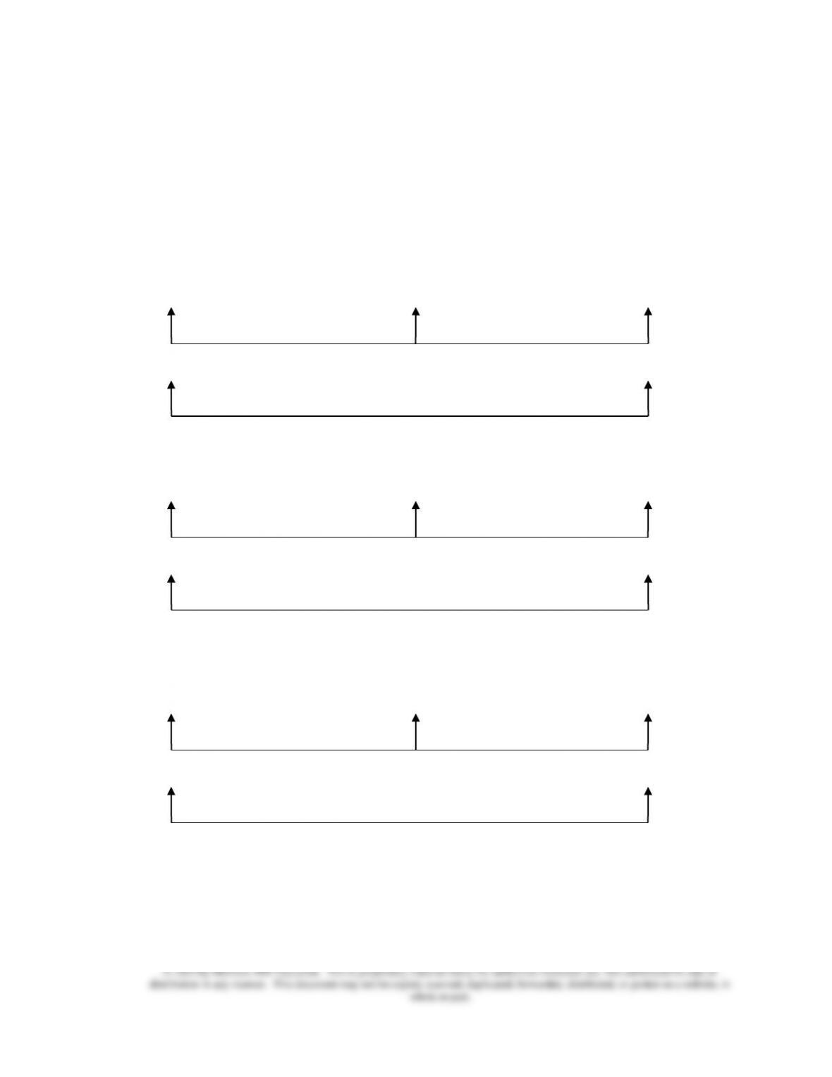
For Bear,
Flexible budget
(SCMa × AQ)
(SCM x ASQb)
Master budget
(SCM × SQ)
$8 × 3,000 = $24,000 $8 × (.25 × 8,000) = $16,000 $8 × 2,500 = $20,000
Mix Variance = $8,000 F Quantity variance = $4,000 U
Activity Variance = $4,000 F
For Monkey,
$4 × 5,000 = $20,000 $4 × (.75 × 8,000) = $24,000 $4 × 7,500 = $30,000
Mix Variance = $4,000 U Quantity variance = $6,000 U
Activity Variance = $10,000 U
For the Stuffed Animals Division as a whole,
$44,000 $40,000 $50,000
Mix Variance = $4,000 F Quantity variance = $10,000 U
Activity Variance = $6,000 U
a SCM = Standard unit contribution margin.
b ASQ = Quantity that would have been sold at the standard mix.
======================

Chapter 17 – Additional Topics in Variance Analysis
17–13
LO 17-4 Evaluate production performance using production mix and yield
variances.
♦ The analysis of mix and quantity variances for sales can be applied to production as well.
• The direct materials efficiency variance can be divided into two components: mix and
yield.
• A production mix variance arises from a change in the relative proportion of inputs (a
materials or labor mix variance).
Production mix
variance
=
Standard input
price
×
(Actual quantity – Actual input
used at the standard mix).
• The production mix variance measures the impact of substitution.
• A production yield variance measures the difference between expected output from a
given level of inputs and the actual output obtained from those inputs.
Production
yield variance
=
Standard input
price
×
(Actual input used at the standard
mix – Standard input allowed).
• The production yield variance measures the input-output relationship holding the
standard mix inputs constant.
• By separating the efficiency variance into its mix and yield components, the pure mix
effect is isolated by holding constant the yield effect, and the pure yield effect is isolated
by holding constant the mix effect.
• See Exhibit 17.6 for an example.
======================
Demonstration Problem 6
Beautiful Paints Company makes different paints. Its semi-gloss paint product requires two
chemical ingredients, X and Y. The standard cost and quantity data follow.
Direct
materials
Standard
price per
gallon
Standard quantity (gallon)
of input per gallon of semi-
gloss paint
Standard cost per
gallon of semi-
gloss paint
Chemical X
$8
.5
$4
Chemical Y
2
.5
1
Chapter 17 – Additional Topics in Variance Analysis
17–14
During October, Beautiful Paints Company had the following results:
Units produced
20,000 gallons of semi-gloss paint
Materials purchased and used
Chemical X
9,800 gallons at $8.20 per gallon
Chemical Y
10,500 gallons at $2.10 per gallon
Required:
Determine the price, mix, and yield variances for Beautiful Paints Company’s semi-gloss
paint in October.
Solution:
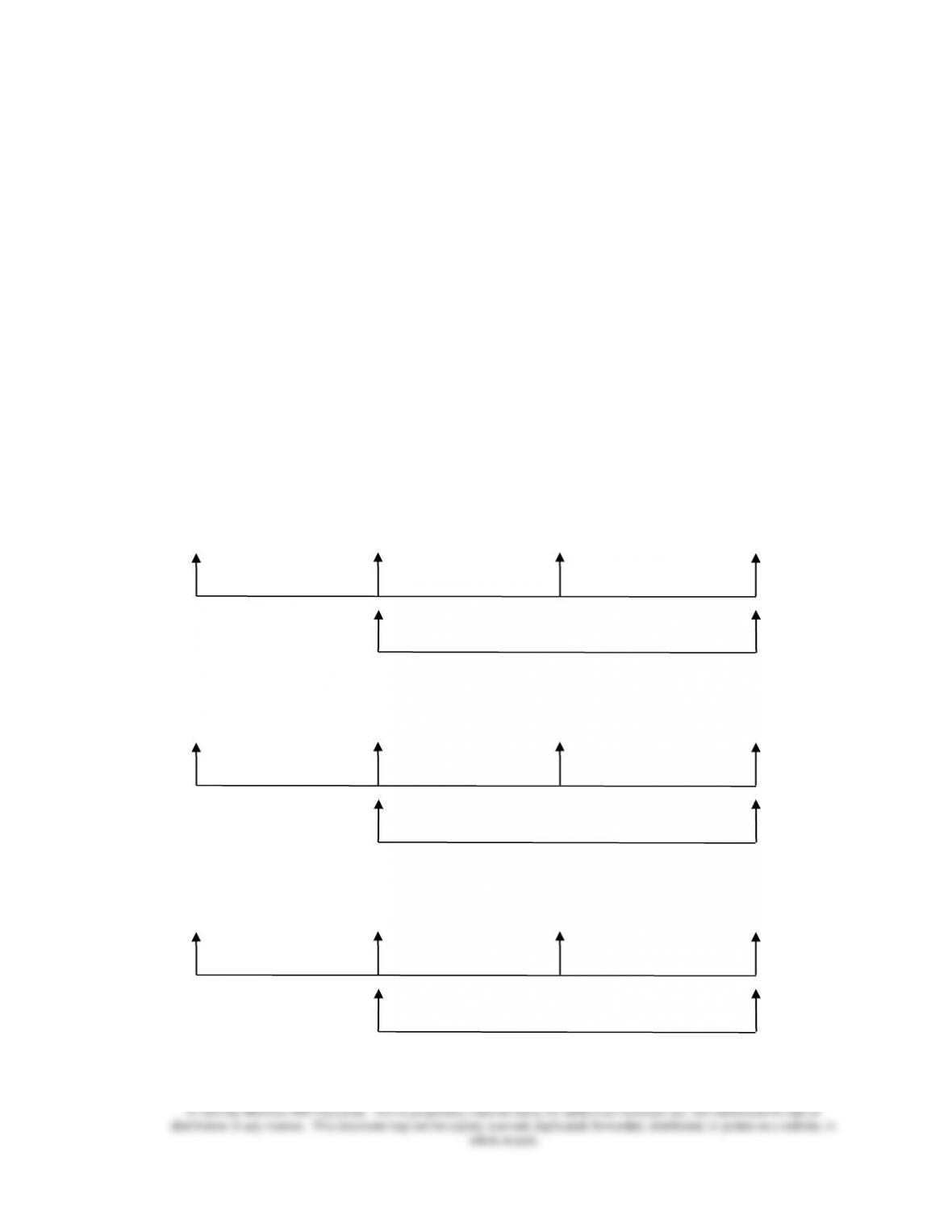
For Chemical X,
Actual
(AP × AQ)
(SP × AQ)
(SP × ASQa)
Flexible budget
(SP × SQ)
Purchase price
variance Mix variance Yield variance
$8.20 × 9,800 = $80,360
$8 × 9,800 = $78,400
$8 × (.5×20,300) = $81,200
$8 × 10,000 = $80,000
$1,960 U $2,800 F $1,200 U
$1,600 F
For Chemical Y,
$2.10 × 10,500 = $22,050
$2 × 10,500 = $21,000
$2 × (.5×20,300) = $20,300
$2 × 10,000 = $20,000
$1,050 U $700 U $300 U
$1,000 U
For the semi-gloss paint,
$102,410
$99,400
$101,500
$100,000
$3,010 U $2,100 F $1,500 U
$600 F
a ASQ = Quantity that would have been sold at the standard mix.

Chapter 17 – Additional Topics in Variance Analysis
17–15
======================
LO 17-5 Apply the variance analysis model to nonmanufacturing costs.
♦ The comparison of the master budget, the flexible budget, and actual results can also be used in
service and merchandising organizations.
• Output is usually defined as sales units in merchandising, but service organizations use
other measures, such as professional staff hours (accounting firms), room nights or guests
(hotels), seat miles or revenue miles (airlines), and patient days (hospitals).
• Merchandising and service organizations focus on marketing and administrative costs to
measure efficiency and control costs.
• The key items to control are labor costs (for service organizations), and occupancy costs
per sales dollar (for merchandising organizations).
• The computation of efficiency variance requires a reliable measure of output activity
that is linked to input.
• In general, jobs with routine tasks lend themselves to efficiency measures, and jobs with
nonroutine tasks do not.
• By substituting different types of labor, service organizations need to calculate labor
mix and yield variances.
• Two factors are important when considering mix variances.
(1) There is an assumed substitutability of inputs.
(2) The input costs must be different for a mix variance to exist.
Chapter 17 – Additional Topics in Variance Analysis
17–16
Demonstration Problem 7
A CPA firm is to perform an audit job for a regular client. Based on past experiences working
with the client, 750 partner hours (at a cost of $200 per hour) and 2,250 staff hours (at a cost of
$75 per hour) are budgeted for the job.
Due to unforeseen events at the client’s sites, a total of 2,700 hours are used consisting of 900
partner hours and 1,800 staff hours. The hourly rate for partner time is the same as budgeted but
the hourly rate for staff time become $100 per hour because more experienced staff members are
put to work.
Required:
Determine all the variances for the CPA firm on the audit job.
Solution:
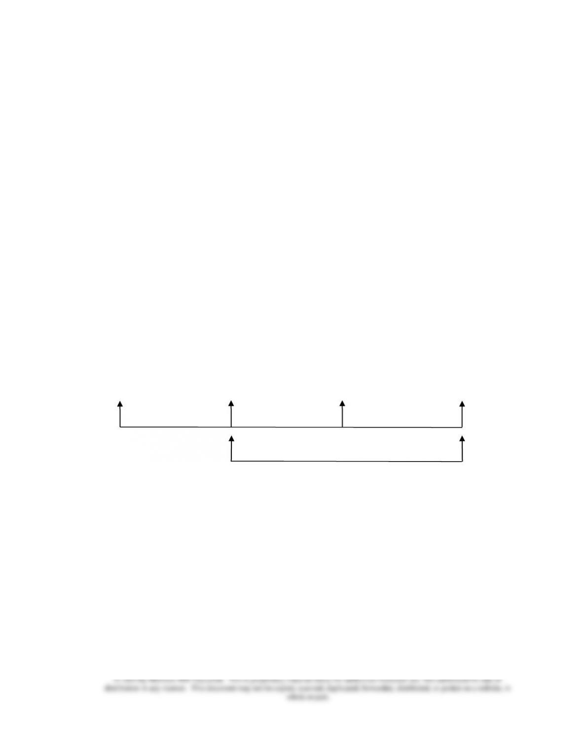
Actual
(AP × AQ)
(SP × AQ)
(SP × ASQa)
Flexible budget
(SP × SQ)
Labor price
variance Mix variance Yield variance
$200 × 900 +
$200 × 900 +
$200 × 675 +
$200 × 750 +
$100 × 1,800 = $360,000
$75 × 1,800 = $315,000
$75 × 2,025 = $286,875
$75 × 2,250 = $318,750
$45,000 U $28,125 U $31,875 F
$3,750 F
a ASQ = Labor hours that would have been used at the standard mix.
2,700 × ¼ = 675; 2,700 × ¾ = 2,025.
A total of 3,000 audit hours are budgeted for the job. The standard mix calls for three staff
hours for each partner hour performed (2,250 ÷ 750 = 3). The actual audit takes 2,700 hours
in which each partner hour is supported by only two staff hours due to staff members’
seniority and experiences.
======================

Chapter 17 – Additional Topics in Variance Analysis
17–17
LO 17-6 Determine which variances to investigate.
♦ Managers and accountants in each organization should perform their own cost-benefit analysis
to ascertain which calculations of variances are justified.
• The variances that will be important for a particular company depend on the strategic
imperatives for the company.
• Impact represents the likely monetary effect from an activity (such as a variance). The
question to ask is, “Does this variance matter?”
• Controllability is the extent to which an item can be managed. The question to ask is,
“Can we do something about it?”
• High-impact, highly controllable variances (such as materials and labor efficiency
variances) should get the most attention.
• Low-impact, uncontrollable variances should get the least attention.
• The longer the time interval is considered, the greater is the ability to control an item.
♦ After computing variances, managers and accountants must decide which ones to investigate.
• Only the variances for which the benefits of correction exceed the costs of follow-up
should be pursued.
• Management by exception is an approach to management requiring that reports
emphasize the deviation from an accepted base point, such as a standard, a budget, an
industry average, or a prior period experience.
• Some problems are easily corrected as soon as they are discovered. The investigation
cost is low and the benefits are very likely to exceed the costs.
• Some variances are not controllable in the short run. Such variances sometimes prompt
long-run actions. In such case, the short-run benefits of variance investigation are low,
but the long-run benefits could be higher.
• Many variances occur because of errors in recording, bookkeeping adjustments, or
timing problems. The accounting staff must carefully check variance reports before
sending them to operating managers.
♦ Standards are estimates that require updating to reflect current conditions.