
Chapter 17 – Additional Topics in Variance Analysis
17-1
Chapter 17
Additional Topics in Variance Analysis
Learning Objectives
1. Explain how to prorate variances to inventories and cost of goods sold.
2. Use market share variances to evaluate marketing performance.
3. Use sales mix and quantity variances to evaluate marketing performance.
4. Evaluate production performance using production mix and yield variances
5. Apply the variance analysis model to nonmanufacturing costs.
6. Determine which variances to investigate.
Chapter Outline
I. PROFIT VARIANCE ANALYSIS WHEN UNITS PRODUCED DO NOT EQUAL
UNITS SOLD
♦ Reconciling variable costing budgets and full-absorption income statements
II. MATERIALS PURCHASES DO NOT EQUAL MATERIALS USED
III. MARKET SHARE VARIANCE AND INDUSTRY VOLUME VARIANCE
IV. SALES ACTIVITY VARIANCES WITH MULTIPLE PRODUCTS
A. Evaluating product mix
B. Evaluating sales mix and sales quantity
• Sources of the sales mix variance
V. PRODUCTION MIX AND YIELD VARIANCES
♦ Mix and yield variances in manufacturing
VI. VARIANCE ANALYSIS IN NONMANUFACTURING SETTINGS
A. Using the profit variance analysis in service and merchandise organizations
B. Efficiency measures
C. Mix and yield variances in service organizations
VII. KEEPING AN EYE ON VARIANCES AND STANDARDS
A. How many variances to calculate
B. When to investigate variances
C. Updating standards
VIII. SUMMARY

Chapter 17 – Additional Topics in Variance Analysis
17-2
Key Concepts
LO 17-1 Explain how to prorate variances to inventories and cost of goods
sold.
♦ The analysis of variances becomes more complicated when the units sold do not equal the units
produced (i.e., when inventory is present).
• The assumption that production was greater than sales has no effect on the sales activity
variance because the master budget and flexible budget are based on sales volume. So are
the sales price variance, and marketing and administrative variances in general.
• In the time period in which units are produced, the variable production cost variance is
calculated as follows:
Variance = (Actual variable cost – Estimated variable cost) × Units produced.
• The actual variable production costs are really a hybrid.
Actual variable
production costs
=
Flexible budget variable
production costs
+ (or -)
Variable production
cost variances.
======================
Demonstration Problem 1
(Revised from Chapter 16 Demonstration Problem 1)
The accountant at EZ Toys, Inc. is analyzing the production and cost data for its Trucks Division.
For October, the actual results and the master budget data are presented below.
Actual results
Budget data
12,000 trucks produced
10,000 trucks sold
12,000 trucks planned
Unit selling price
$15
Unit selling price
$14
Unit variable costs:a
Unit variable cost:
Direct materials
$5.28
Direct materials
$5
Direct labor
5.10
Direct labor
4
Variable overhead
2.30
Variable overhead
2
Total variable costs
$12.68
Total unit variable costs
$11
Fixed overhead
$9,000
Fixed overhead
$9,600
a These are average costs.

Chapter 17 – Additional Topics in Variance Analysis
17-3
Required:
Prepare a profit variance analysis.
Solution:
Actual
(based on
actual
activity of
10,000 units
sold)
Manufacturing
variances
Sales price
variance
Flexible
budget
(based on
actual
activity of
10,000 units
sold)
Sales
activity
variance
Master
budget
(based on
12,000
units
planned)
Sales revenue
$150,000
$10,000 F
$140,000
$28,000 U
$168,000
Less: Costs
Variable costs
Direct materials
$53,360
$3,360 Ua
$50,000
$10,000 F
$60,000
Direct labor
53,200
13,200 Ub
40,000
8,000 F
48,000
Variable overhead
23,600
3,600 Uc
20,000
4,000 F
24,000
Total variable costs
$130,160
$110,000
$22,000 F
$132,000
Contribution margin
$19,840
$30,000
$6,000 U
$36,000
Fixed overhead
9,000
600 F
9,600
0
9,600
Operating profit
$10,840
$19,560 U
$10,000 F
$20,400
$6,000 U
$26,400
F = Favorable variance.
U = Unfavorable variance.
a 12,000 × ($5.28 – $5) = $3,360 U.
b 12,000 × ($5.10 – $4) = $13,200 U.
c 12,000 × ($2.30 – $2) = $3,600 U.
======================
• The entire variable production cost variance for units produced can be treated as a period cost
and expensed in the period incurred, or it can be prorated between units sold and units still in
inventory.
Cost of goods sold
xx
Fixed overhead price variance
xx
Fixed overhead production volume variance
xx
Variable production cost variances
xx
(To close production cost variances to Cost of goods sold; the debits and credits are
assumed)

Chapter 17 – Additional Topics in Variance Analysis
17-4
Cost of goods sold
xx
Finished goods inventory
xx
Fixed overhead price variance
xx
Fixed overhead production volume variance
xx
Variable production cost variances
xx
(To close production cost variances to Cost of goods sold and Finished goods inventory;
the debits and credits are assumed)
• Using variable costing, the entire fixed production cost is expensed when incurred.
• When standard, full-absorption costing is used and production and sales volumes are
not the same, the profit reported will be different from that reported under variable
costing (due to the accounting system, not managerial efficiency). Care must be taken to
identify the cause of such profit differences.
• Exhibit 17.2 reconciles the reported income statement under full absorption with that
under variable costing.
======================
Demonstration Problem 2
(Continued from Demonstration Problem 1)
Required:
Reconcile reported income using standard, full-absorption costing with that using standard,
variable costing for the Trucks Division of EZ Toys in October.

Chapter 17 – Additional Topics in Variance Analysis
17-5
Solution:
Actual
(using
standard, full-
absorption
costing)
Inventory
adjustment
Actual
(using
standard,
variable
costing)
Sales revenue
$150,000
$150,000
Less:
Variable costs
Direct materials (at standard)
$50,000
$50,000
Direct labor (at standard)
40,000
40,000
Variable overhead (at standard)
20,000
20,000
Variable production cost variances (net)
20,160a
20,160
Less:
Fixed overhead
8,000
$(1,600)
9,600
Fixed overhead variance (net)
(600)
(600)
Operating profit
$12,440
$(1,600)
$10,840
a $3,360 U + $13,200 U + $3,600 U = $20,160 U.
Using variable costing, the entire fixed production cost of $9,000 is expensed in October.
Under standard, absorption costing, each truck is allocated fixed production cost of $0.80
(= $9,600 ÷ 12,000 units). A portion of the fixed production cost is allocated to the 2,000
units in ending inventory:
$0.80 × 2,000 = $1,600.
Thus, only $7,400 (= $9,000 – $1,600) of the actual fixed production cost are expensed in
October under standard, full-absorption costing. This includes $8,000 (= $0.80 × 10,000 units)
of fixed production cost in standard cost of goods sold plus a favorable budget variance of
$600.
In this case, full-absorption operating profit would be $12,440, or $1,600 higher than variable
costing operating profit. The $1,600 difference in profits is due to the accounting system, not
because of operating activities.
======================
♦ When the quantities of materials purchased and used are not the same, a purchase price
variance based on the quantity of materials purchased can be calculated.
Purchase price variance = (Actual price – Standard price) × Actual quantity purchased.

Chapter 17 – Additional Topics in Variance Analysis
17-6
• The materials efficiency variance remains the same because it is based on materials
used.
• One advantage of using a standard costing system is that managers receive information
that is useful in making decisions to improve performance.
• The sooner the information is received (such as information about the purchase price
variance shortly after the acquisition of materials), the sooner it can be used for decision
making purposes.
• If materials are stored, recording the purchase at standard cost provides information on
price variances earlier than if the firm waits until the materials are used.
======================
Demonstration Problem 3
(Revised from Chapter 16 Demonstration Problem 3)
Information about the use of direct materials at EZ Toys’ Trucks Division for October is as
follows:
Standard costs
2 units per truck @ $2.50 per unit
=
$5 per truck
Trucks produced in October
=
10,000
Actual materials purchased
23,200 units @ $2.40 per unit
=
$55,680
Actual materials used
22,000 units @ $2.40 per unit
=
$52,800
There was no beginning inventory on October 1.
Required:
Prepare the Truck Division’s direct materials variances for October.
Chapter 17 – Additional Topics in Variance Analysis
17-7
Solution:
Actual costs =
Actual input quantity
at actual input price
$2.40 × 23,200 =
$55,680
Actual input quantity at
standard input price
$2.50 × 23,200 =
$58,000
Flexible production budget =
Standard input quantity allowed
for actual output at standard
input price
Price Variance
$2,320 F
$2.50 × 22,000 = $55,000 $2.50 × 20,000 = $50,000
Efficiency Variance
$5,000 U
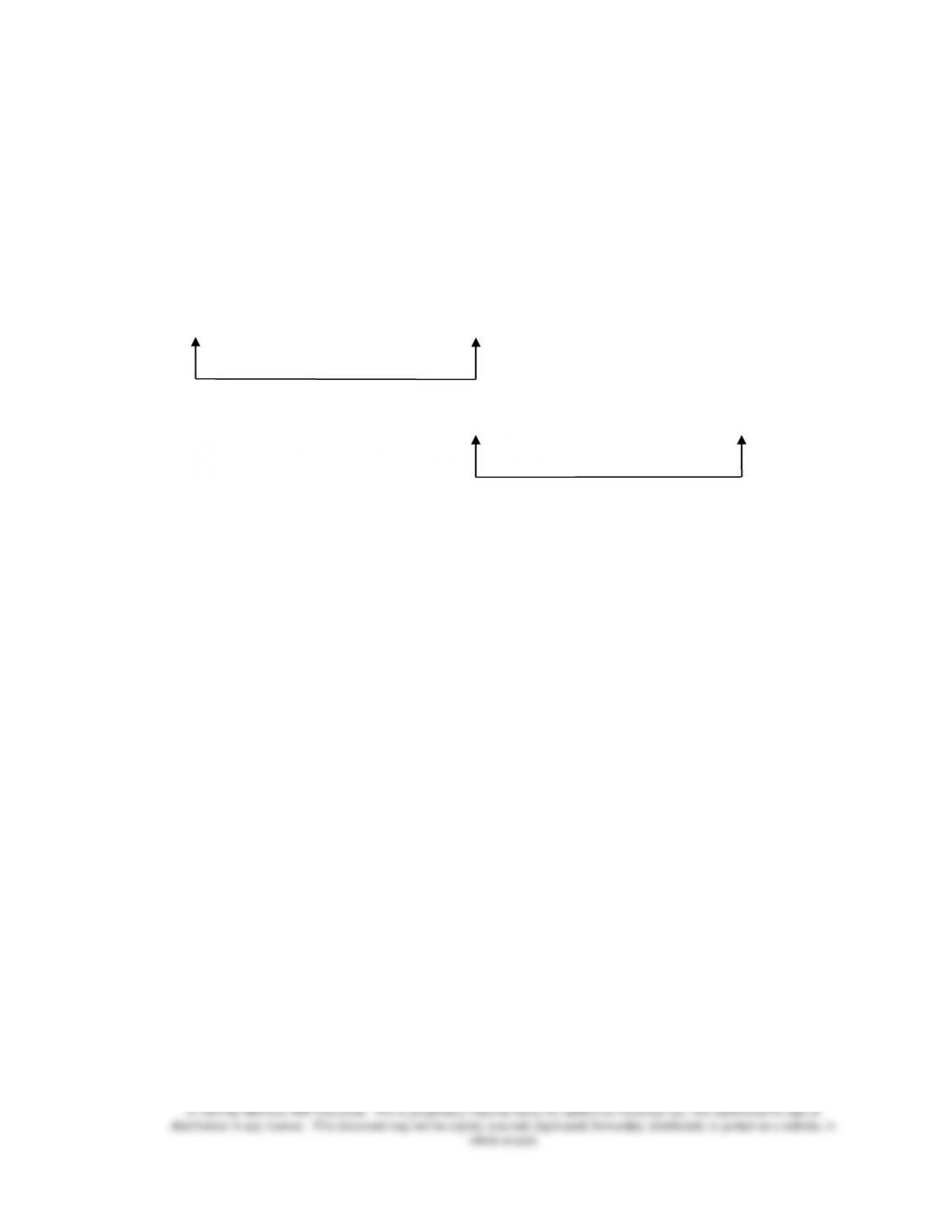
The price variance is based on the quantities purchased (23,200 units), while the efficiency
variance is based on the quantities used (22,000 units vs. 20,000 units allowed under the flexible
budget).
======================
• The relevant journal entries are
Materials inventory
xx
Material price variance
xx
Accounts payable
xx
(To record materials purchase and material price variance; Unfavorable variance is
assumed).
Work in process inventory
xx
Material efficiency variance
Materials inventory
xx
(To record the use of materials and material efficiency variance; Unfavorable variance is
assumed).

Chapter 17 – Additional Topics in Variance Analysis
17-8
LO 17-2 Use market share variances to evaluate marketing performance.
♦ The general approach in variance analysis is to separate the variance into components based on
a budgeting formula.
• The same idea is applicable to variances in sales activities.
♦ Many companies base an initial sales forecast on an estimate of sales activity in the industry as
a whole and on an estimate of the company’s market share.
• There are two reasons why actual sales activity is different from budgeted sales activity:
(1) Actual industry volume was different from budgeted industry volume, and/or
(2) Actual market share was different from budgeted market share.
• Industry volume variance represents the portion of the sales activity variance
attributable to changes in industry volume.
• Market share variance represents the portion of the sales activity variance due to
changes in the company’s proportion of sales in the markets in which the company
operates.
• By decomposing sales activity variance into an industry volume and a market share
variance, management has additional information that can be used to make operational
improvements next period.
• Multiplying each figure (one from the industry effect, the other from the market share
effect) by the standard contribution margin gives the impact of these variances on
operating profit. That is,
Industry
volume
variance
=
Standard
contribution
margin per unit
×
(Actual industry volume –
Budgeted industry volume)
×
Budgeted
market share.
Market
share
variance
=
Standard
contribution
margin per unit
×
Actual industry
volume
×
(Actual market share –
Budgeted market share).

Chapter 17 – Additional Topics in Variance Analysis
17-9
Example: Pioneer Uniform, Inc. serves two groups of the customers in the market,
Retail and Commercial. The following budget information is available for June.
Customers
Unit
contribution
margin
Sales
volume
Sales
mix
Commercial
$5
40,000
80%
Retail
8
10,000
20%
50,000
Since two “products” are offered in the same industry, a composite (weighted-average)
standard contribution margin per unit needs to be calculated to determine the industry
volume and market share variances later. The weights are based on the standard sales
mix.
Composite standard contribution margin per unit = $5 × 80% + $8 × 20% = $5.60.
• The market share variance is usually more controllable by the marketing department
and is a measure of its performance.
• The use of the industry volume and market share variances enables management to
separate that portion of the activity variance that coincides with changes in the overall
industry from that which is specific to the company.
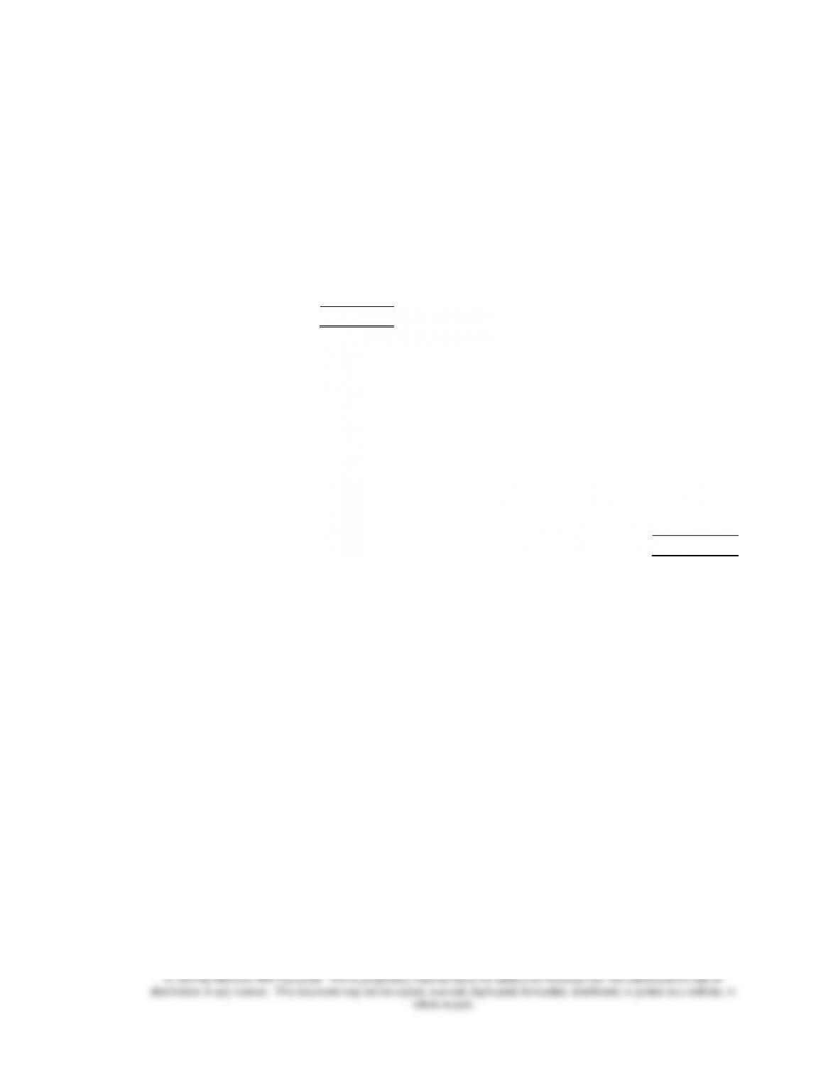
• Exhibit 17.4 illustrates the relation between these two market-related variances.
======================
Demonstration Problem 4
(Continued from Demonstration Problem 1)
EZ Toys’ marketing manager estimated the sales of 12,000 trucks in October for the Trucks
Division based on an estimated industry volume of 80,000 trucks and on the Trucks Division’s
ability to maintain a market share of 15 percent in the past. That is,
80,000 trucks to be sold in the market × 15% of estimated market share = 12,000 trucks.
Due to unexpected shift in demand, the industry volume in toy truck sales dropped to 62,500
units in October while EZ Toys’ Trucks Division managed to sell a total of 10,000 units.
Chapter 17 – Additional Topics in Variance Analysis
17–10
The following information is also available.
Budget data
Unit selling price
$14
Unit variable cost:
Direct materials
$5
Direct labor
4
Variable overhead
2
Total unit variable costs
$11
Required:
Prepare October’s industry volume and market share activity variances for the Trucks
Division of EZ Toys.
Solution:
The Trucks Division’s actual market share for October was 16% (= 10,000 units ÷ 62,500
units).
Industry volume variance
($14 – $11) × (62,500 units – 80,000 units) × 15%
=
$7,875 U
Market share variance
($14 – $11) × 62,500 units × (16% – 15%)
=
1,875 F
Sales activity variance
$6,000 U
======================
LO 17-3 Use sales mix and quantity variances to evaluate marketing
performance.
♦ The sales activity variance can be divided into two components: sales mix and sales quantity.
• A sales mix variance arises from the relative proportion of different products sold,
holding constant the quantity effects.
Sales mix
variance
=
Standard contribution
margin per unit
×
(Actual quantity sold – Quantity that would
have been sold at the standard mix).
• A sales mix variance provides useful information for a company that sells multiple
products when these products are (imperfect) substitutes for each other.
• The sales mix variance measures the impact of substitution.