Chapter 16 – Fundamentals of Variance Analysis
16–11
• Managers who are responsible for price variances would not be held responsible for
efficiency variances and vice versa.
• The total cost variance is the difference between budgeted and actual results (equal to
the sum of the price and efficiency variances).
Total cost variance = (AP × AQ) – (SP × SQ).
• The general model is applied to each variable cost incurred and is outlined in Exhibit
16.7. That is,
Actual costs =
Actual input quantity
at actual input price
(AP x AQ)
Actual input
quantity at standard
input price
(SP x AQ)
Flexible production budget =
Standard input quantity allowed
for actual output at standard
input price
(SP x SQ)
Price (Rate, or Spending) Quantity (Usage, or Efficiency)
Variance Variance
(AP – SP) × AQ SP × (AQ – SQ)
Total cost variance
(AP × AQ) – (SP × SQ)
• The comprehensive cost variance analysis will ultimately explain, in detail, the variable
manufacturing cost variance calculated earlier.
• A flexible production budget is calculated as standard input price times standard
quantity of input allowed for actual good output. It is based on actual production volume.
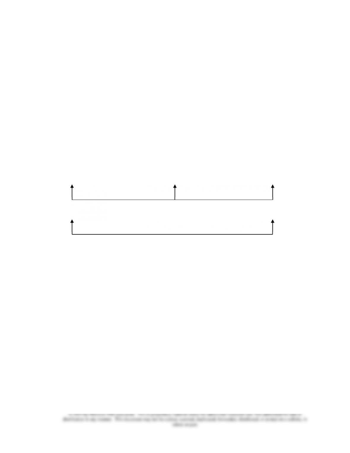
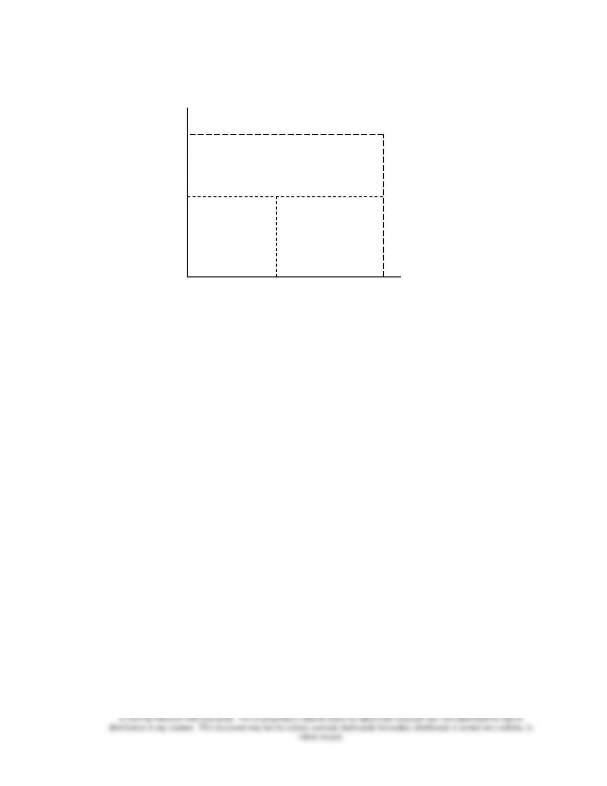
• An alternative way to view these variances graphically is shown below. Quantities are
presented on the horizontal axis and prices on the vertical axis. The three areas are
standard cost (SP × SQ), price variance ((AP – SP) × AQ), and efficiency variance (SP ×
(AQ – SQ)), respectively.
Chapter 16 – Fundamentals of Variance Analysis
16–12
♦ Exhibit 16.8 applies the general model to direct materials variances.
• Responsibility for the direct materials price variance is usually assigned to the
purchasing department.
• Explanations for a materials price variance include failure to take purchase discounts,
higher transportation costs than expected, different grade of direct materials purchased, or
changes in the market price of direct materials.
• Direct materials efficiency variances are typically the responsibility of production
departments and may be due to defects in direct materials, inexperienced workers, poor
supervision, and so on.
======================
Demonstration Problem 3
(Continued from Demonstration Problem 1)
Information about the use of direct materials at EZ Toys’ Trucks Division for October follows:
Standard costs
2 units per truck @ $2.50 per unit
=
$5 per truck
Trucks produced in October
=
10,000
Actual materials purchased and used
22,000 units @ $2.40 per unit
=
$52,800
There was no beginning inventory on October 1.
Standard Cost
= SP × SQ
Efficiency Variance
= SP × (AQ – SQ)
Price Variance
= (AP – SP) × AQ
SQ
AQ
SP
AP
Quantities
Prices
Chapter 16 – Fundamentals of Variance Analysis
16–13
Required:
Prepare the Truck Division’s direct materials variances for October.
Solution:
Actual costs =
Actual input quantity
at actual input price
$2.40 × 22,000 = $52,800
Actual input quantity at
standard input price
$2.50 × 22,000 = $55,000
Flexible production budget =
Standard input quantity allowed
for actual output at standard
input price
$2.50 × 20,000 = $50,000
Price Variance Efficiency Variance
$2,200 F $5,000 U
Total cost variance
$2,800 U
======================
♦ Exhibit 16.9 applies the general model to direct labor variances.
• The direct labor price variance may be caused by hiring less experienced employees.
• If the wage rates used in setting standards are the same as those in the union contract,
labor price variances will not occur.
• The labor efficiency variance is a measure of labor productivity and is usually
controlled by production managers.
• Unfavorable labor efficiency variances may be due to poorly motivated or trained
workers, poor materials or faulty equipment, poor supervision and scheduling problems.
• One event, such as hiring inexperienced employees, can affect more than one variance.
======================
Demonstration Problem 4
(Continued from Demonstration Problem 1)
Information about the use of direct labor at EZ Toys’ Trucks Division for October follows:
Chapter 16 – Fundamentals of Variance Analysis
16–14
Standard costs
0.4 hour per truck @ $10 per hour
=
$4 per truck
Trucks produced in October
=
10,000
Actual direct labor costs
Actual hours worked
=
5,000
Total actual labor cost
=
$51,000
Average cost per hour
=
$10.20
Required:
Prepare the Truck Division’s direct labor variances for October.
Solution:
Actual costs =
Actual input quantity
at actual input price
$10.20 × 5,000 = $51,000
Actual input quantity at
standard input price
$10 × 5,000 = $50,000
Flexible production budget =
Standard input quantity allowed
for actual output at standard
input price
$10 × 4,000 = $40,000
Price Variance Efficiency Variance
$1,000 U $10,000 U
Total cost variance
$11,000 U
======================
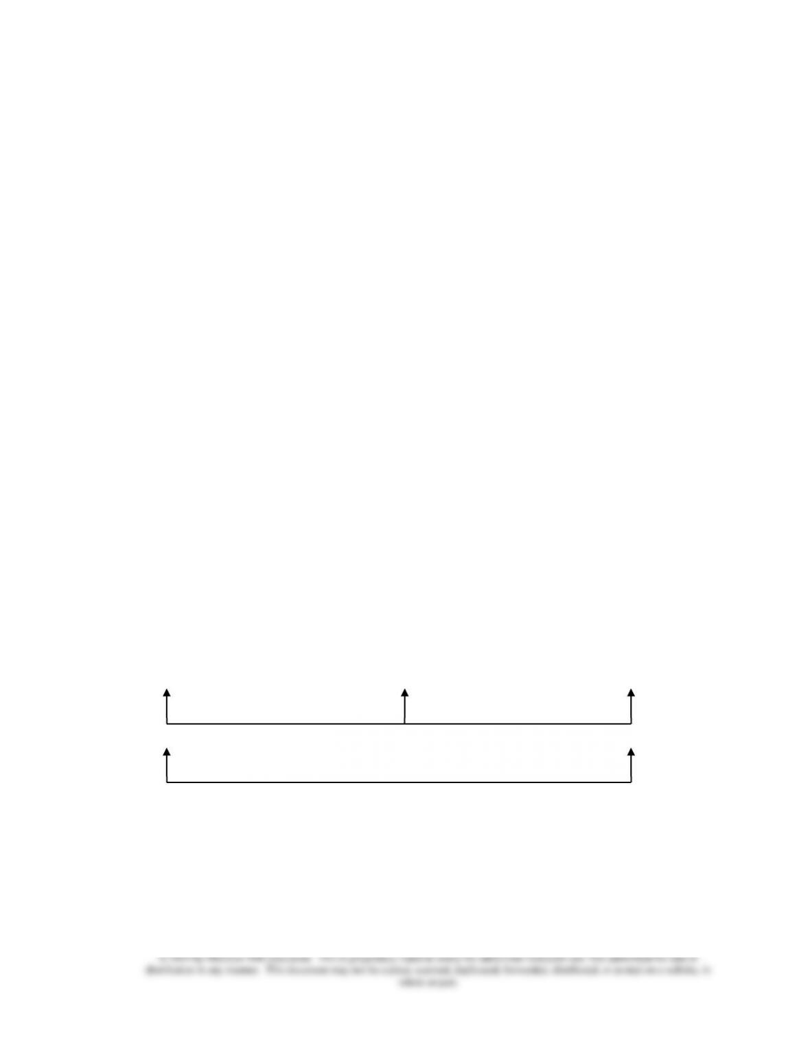
♦ Exhibit 16.10 applies the general model to variable overhead variances.
• The variable overhead standard rate is derived from a two-stage estimation of
(1) costs at various levels of activity, and
(2) the relationship between those estimated costs and the basis.
• The variable overhead price variance could have occurred because
(1) actual costs are different from those expected, and
(2) the relationship between variable production overhead costs and the basis chosen is
not perfect.
• The variable overhead price variance actually contains some efficiency items as well as
price items. Some companies separate those components.
Chapter 16 – Fundamentals of Variance Analysis
16–15
• The variable overhead efficiency variance is not related to the use (or efficiency) of
variable overhead. Instead, it is related to efficiency in using the base on which variable
overhead is applied.
• Managers who are responsible for controlling the base will probably be held responsible
for the variable overhead efficiency variance as well.
======================
Demonstration Problem 5
(Continued from Demonstration Problem 1)
Information about the use of variable overhead at EZ Toys’ Trucks Division for October follows:
Standard costs
0.4 hour per truck @ $5 per hour
=
$2 per truck
Trucks produced in October
=
10,000
Actual variable overhead cost
=
$23,000
Required:
Prepare the Truck Division’s variable overhead variances for October.
Solution:
Actual costs =
Sum of actual variable
overhead costs
$23,000
Actual input quantity at
standard input price
$5 × 5,000 = $25,000
Flexible production budget =
Standard input quantity allowed
for actual output at standard
input price
$5 × 4,000 = $20,000
Price Variance Efficiency Variance
$2,000 F $5,000 U
Total cost variance
$3,000 U
======================
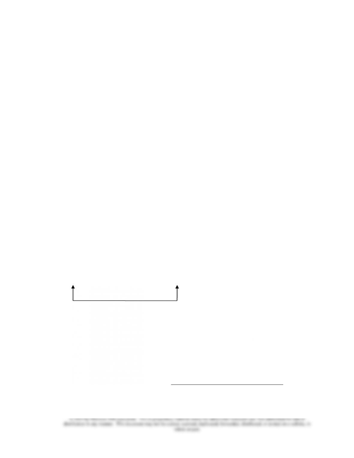
♦ Exhibit 16.11 summarizes the variable production cost variances.
• A summary of this nature is useful for reporting variances to high-level managers. It
provides both an overview of variances and their sources.
Chapter 16 – Fundamentals of Variance Analysis
16–16
• Management could want more detailed information about some of the variances by
extending each variance branch to show variances by product line, department, or other
categories.
LO 16-6 Compute and use fixed cost variances.
♦ It is usually assumed that fixed costs are unchanged when volume changes within the relevant
range, so the amount budgeted for fixed overhead is the same in both the master and flexible
budgets.
• Fixed costs are period costs by nature.
• When the income statement is prepared using variable costing, there is no absorption of
the fixed costs by units of production. All the fixed manufacturing overhead is charged to
income in the period incurred.
• Fixed overhead has no input-output relationships and, therefore, no efficiency variance.
• A spending (or budget) variance, the price variance for fixed overhead, is the
difference between the flexible budget and the actual fixed overhead and is entirely due
to changes in the costs that make up fixed overhead.
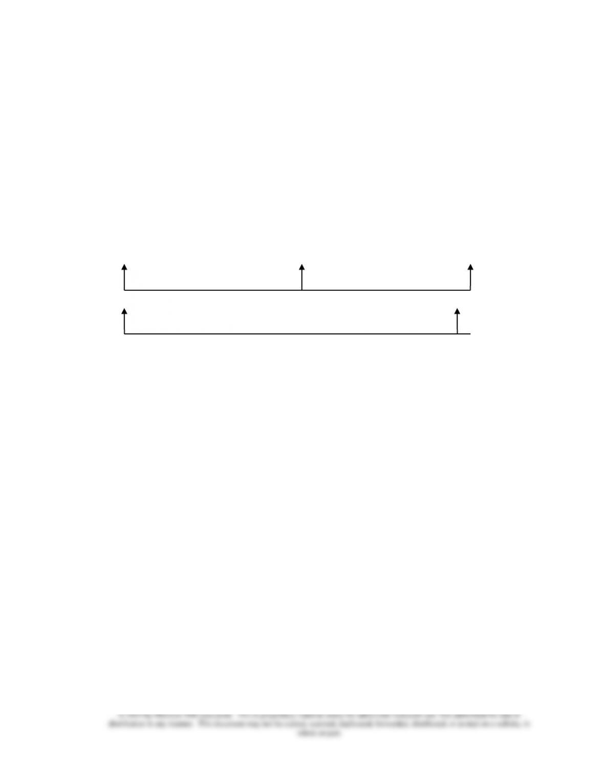
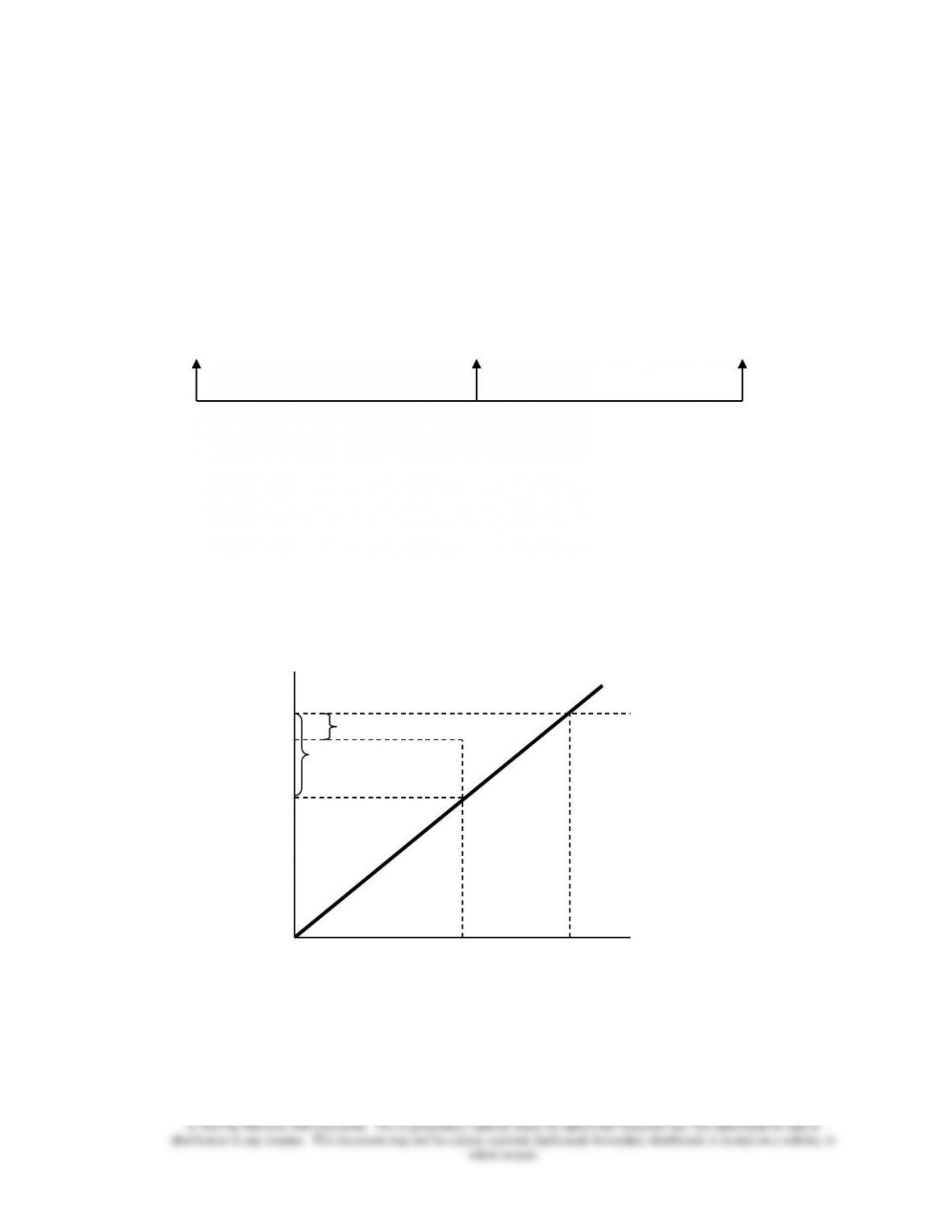
• Exhibit 16.12 shows a variance analysis for fixed overhead. That is,
Actual
Flexible production
budget
Price (spending) variance
(Efficiency variance is not applicable)
♦ When companies use full-absorption, standard costing, fixed production costs are unitized and
treated as product costs.
• The fixed manufacturing standard cost is determined before the start of the production
period using the following formula from Chapter 7:
Standard (or predetermined)
fixed production overhead cost
=
Budgeted fixed manufacturing overhead
Budgeted activity level
.
Chapter 16 – Fundamentals of Variance Analysis
16–17
• A production volume variance (also called capacity variance, idle capacity variance,
or denominator variance) is the difference between the applied fixed overhead and the
budgeted fixed overhead.
• Production volume variances arise because the volume used to apply fixed overhead
differs from the estimated volume used to calculate fixed overhead per unit.
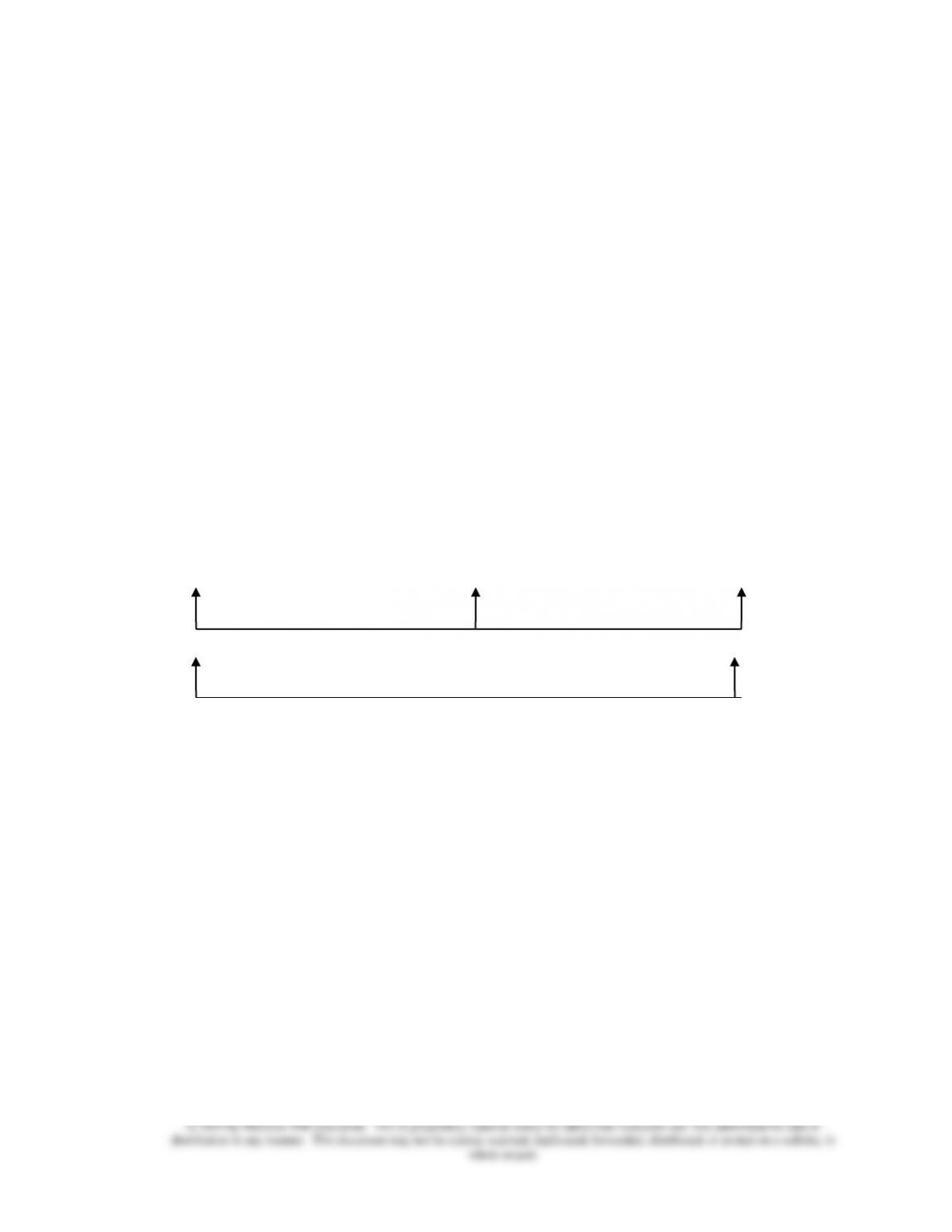
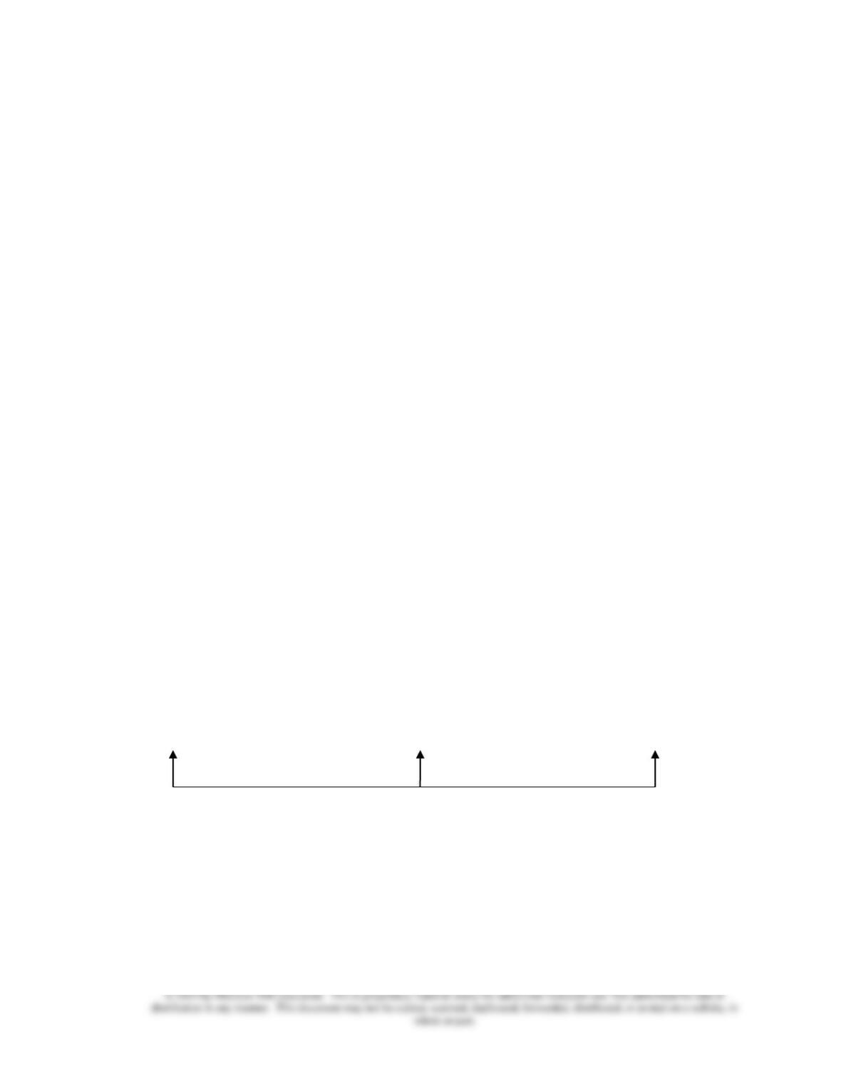
• Exhibit 16.13 demonstrates the variance analysis for fixed overhead under
absorption costing. That is,
Actual
Budgeted
Applied
Price (spending) variance Production volume variance
• An alternative way to present fixed overhead variances graphically is shown below (see
also Exhibit 16-14). Since fixed overhead is unitized through the calculation of
predetermined fixed overhead rate, fixed overhead is applied as if it were variable cost, as
seen in the application line. At the budgeted volume, the applied fixed overhead
coincides with budgeted fixed overhead, as seen in the budget line. Since actual volume
is less than the budgeted volume in this graph, the applied fixed overhead is less than the
budgeted fixed overhead; the difference between the two represents the production
volume variance. The difference between actual and budgeted fixed overhead becomes
the price (or spending) variance.
Application line
Budget line
Actual
volume
Budgeted
volume
Budget
Applied
Actual
Production volume variance
Price (spending) variance
Chapter 16 – Fundamentals of Variance Analysis
16–18
• The production volume variance applies only to fixed costs as a result of allocating a
fixed period cost to units on a predetermined basis. It does not represent resources spent
or saved, and is unique to full-absorption costing.
• The benefits of calculating the production volume variance for control purposes are
questionable.
• The price (spending) variance is used for control purposes because it is a measure of
difference between actual and budgeted period costs.
======================
Demonstration Problem 6
(Continued from Demonstration Problem 1)
Information about the use of fixed overhead at EZ Toys’ Trucks Division follows:
Annual budget data
Fixed overhead
=
$115,200
Direct labor hours
=
57,600
Standard fixed overhead rate
=
$2 per hour
Standard costs
0.4 hour per truck @ $2 per hour
=
$0.80 per truck
Trucks produced in October
=
10,000
Actual variable overhead cost
=
$9,000
Required:
Prepare Truck Division’s fixed overhead variances for October.
Solution:
Actual costs
$9,000
Budgeta
$9,600
Applied
$2 × 4,000 = $8,000
Price Variance Efficiency Variance
$600 F $1,600 U
a $115,200 / 12 months = $9,600 per month.
======================
♦ The method of computing overhead variances described is known as the four-way analysis of
overhead variances because it computes the following four variances: price and efficiency for
variable overhead, and price and production volume for fixed overhead.

Chapter 16 – Fundamentals of Variance Analysis
16–19
• Exhibit 16.15 summarizes the four-way analysis of variable and fixed overhead
variances.
• The variable overhead efficiency variance measures the efficiency in using the
allocation base.
• The production volume variance occurs only when fixed production cost is unitized.
The budgeted fixed overhead might not equal the amount applied to units produced.
• There is no efficiency variance for fixed production costs.
• Managers evaluated by variances that include production volume variance do have an
incentive to overproduce. This is due to how standard costing is usually practiced. See In–
Action item for more information.
LO 16-7 (Appendix) Understand how to record costs in a standard costing
system.
♦ Standard costing is an accounting method that assigns costs to cost objects at predetermined
amounts.
• The entry debiting Work in process inventory at standard cost could be made before
actual costs are known.
• Actual costs are accumulated in accounts such as Accounts payable and Wages payable
and are compared with the standard costs allowed for the output produced.
• The difference between the actual costs assigned to a department and the standard costs
of the work done is the variance for the department.
• Direct materials
Work–in–process inventory
xx
Materials price variancea
xx
Materials efficiency variance
xx
Accounts payable
xx
(To record the purchase and use of materials at actual cost and the transfer to work in
process at standard cost)