Chapter 11 – Service Department and Joint Cost Allocation
11–11
a $240,000 = $1,200,000 × 20.0%.
b $200,000 = $500,000 × 40.0%.
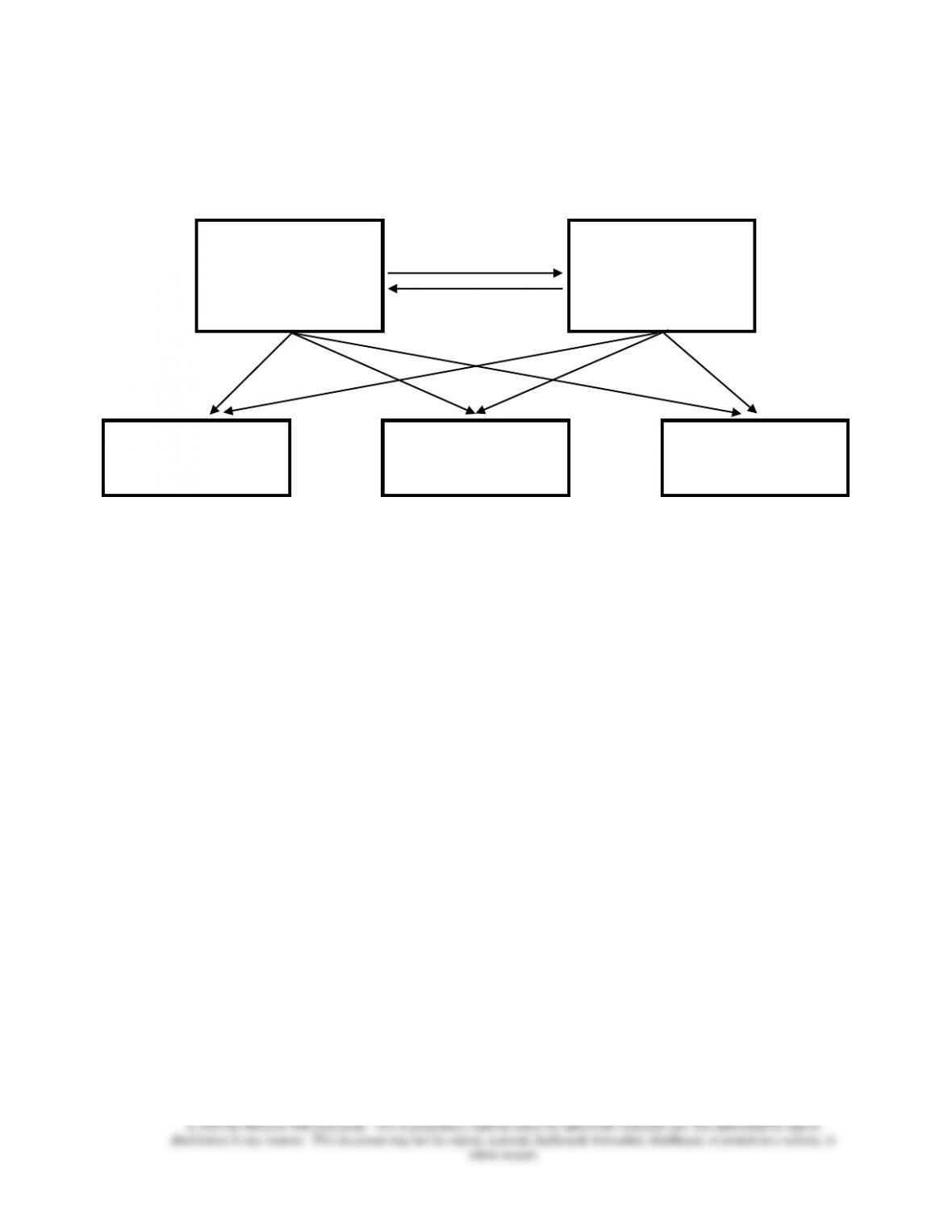
S1
To S2: $240,000
To P1: $360,000
To P2: $480,000
To P3: $120,000
S2
To S1: $200,000
To P1: $100,000
To P2: $75,000
To P3: $125,000
To S2: $240,000
To S1: $200,000
P1
From S1: $360,000
From S2: $100,000
P2
From S1: $480,000
From S2: $75,000
P3
From S1: $120,000
From S2: $125,000
======================
♦ The three service department allocation methods can be compared in two ways.
• The first is to examine how each allocates costs to departments receiving services.
As shown in Exhibit 11.12, only the reciprocal method allocates costs to all departments
receiving services from other departments.
• The second way is to examine the costs each ultimately allocates to manufacturing and
marketing departments, as shown in Exhibit 11.13.
• Each method allocates the same total cost.
• The direct method results sometimes are closer to the reciprocal method results than the
results using the step method.
• All three allocation methods are arbitrary. If one production department stops using the
service of a service department, the costs saved by the firm are unlikely to be equal to the
costs allocated by any of the methods.

Chapter 11 – Service Department and Joint Cost Allocation
11–12
LO 11-5 Use the reciprocal method for decisions.
♦ The primary purpose of allocating service department costs to the production departments is to
obtain the manufacturing costs for each of the production departments for product costing and
inventory valuation.
• The cost information is also developed to assist managers in making decisions, such as
whether to outsource some or all of the activities of the service departments.
• The cost savings will depend on how much an outside vendor will charge and how
much cost in the service departments can be eliminated if outsourced.
• If there are no reciprocal services among the service departments, the cost savings are
the cost of the eliminated service department that is avoidable (= variable costs + any
avoidable fixed costs).
• If there are reciprocal services, the manager has to consider the effect of eliminating one
of the service departments on the service requirements of the remaining service
departments.
• Because the reciprocal method explicitly recognizes the use of one service department
by another, it provides an estimate of what one department costs when reciprocal service
costs are included.
======================
Demonstration Problem 4
(Revised from Demonstration Problem 3)
Kirby Industries is considering the possibility of outsourcing the activities of service department
S1. In order to evaluate the bids from qualified vendors, Kirby’s accountant provides the
following revised data that reflect only the variable costs incurred.
Variable
Proportion of services provided to:
costs
incurred
Service
department
S1
S2
P1
P2
P3
$300,000
S1
–
20%
30%
40%
10%
104,000
S2
40%
–
20%
15%
25%
The avoidable fixed costs of running service department S1 are estimated to be $390,000.

Chapter 11 – Service Department and Joint Cost Allocation
11–13
Required:
Determine the possible cost savings from eliminating service department S1.
Solution:
Define S1 and S2 to be the variable service department costs for departments S1 and S2,
respectively.
The service department S1 incurred $300,000 for providing services to other departments.
The service department S2 provided 40 percent of its services to S1. Together, the total
service department costs for S1 can be expressed as:
S1 = $300,000 + .4 × S2.
The service department S2 incurred $104,000 for providing services to other departments.
The service department S1 provided 20 percent of its services to S2. Together, the total
service department costs for S2 can be expressed as:
S2 = $104,000 + .2 × S1.
Next, insert S1 information into S2. That is,
S2 = $104,000 + .2 × [$300,000 + .4 × S2].
Then,
S2 = $104,000 + $60,000 + .08 × S2.
.92 × S2 = $164,000.
S2 = $178,261.
S1 = $371,304.
The total variable cost of service department S1 is $371,304. This figure includes S1’s direct
cost ($300,000) and 40 percent of S2’s cost ($71,304 = $178,261 × 40%).
Out of the fixed cost of service department S1 of $700,000 (= $1,000,000 total costs –
$300,000 variable costs), $390,000 is estimated to be avoidable.
When managers of Kirby Industries evaluate bids from outside vendors, their benchmark will
be the avoidable costs which can be saved from eliminating service department S1, $761,304
(= $371,304 variable costs + $390,000 avoidable fixed costs).
======================

Chapter 11 – Service Department and Joint Cost Allocation
11–14
Split-off point
LO 11-6 Explain why joint costs are allocated.
♦ Joint cost is a cost of a manufacturing process with two or more different outputs. Joint
products are such outputs from a common input and common production process.
• The problem is whether and how to allocate the joint cost of the input to the joint
products.
• Split-off point is the stage of processing when two or more products are separated.
Processing costs incurred prior to the split-off point are the joint costs.
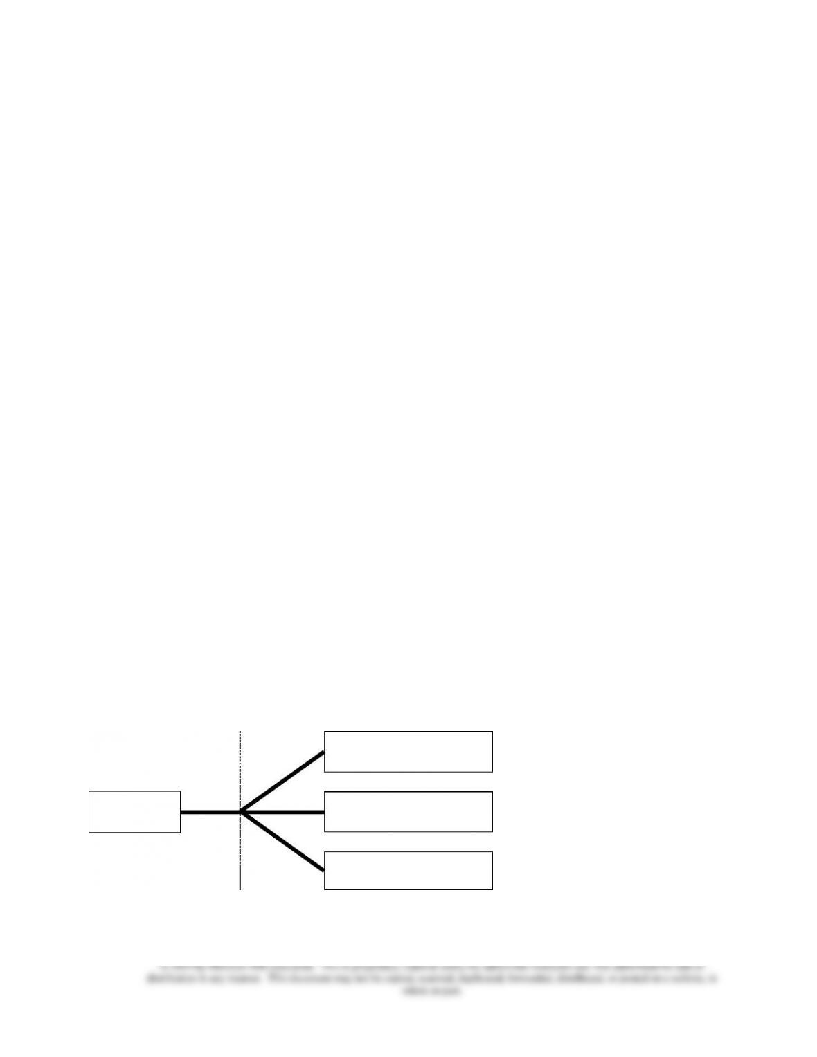
Example 1: The following shows a joint production process and its joint costs. After
the split-off point, two discernable joint products, A and B, emerge from the process.
The costs before the split-off point are joint; any costs spent afterwards are separable.
Joint product A
Raw
materials
Joint production
process
(with additional
materials, labor, and
overhead)
Joint product B
Joint cost
• Exhibit 11.14 shows a diagram of joint cost flows.
• Cost allocations are often used to determine departmental or division costs for
measuring executive performance.
• When a single raw material is converted into products sold by two or more departments,
the cost of the raw material must be allocated to the products involved.
• Manufacturing companies must allocate joint costs to measure the inventory value of
the products that result from the joint process.
Chapter 11 – Service Department and Joint Cost Allocation
11–15
• When companies are subject to rate regulation, the allocation of joint costs can be a
significant factor in determining the regulated rates.
• Any cost allocation method contains an element of arbitrariness and must be clearly
stated before being implemented.
LO 11-7 Allocate joint costs using the net realizable value method.
♦ The two major methods of allocating joint costs are
(1) the net realizable value method, and
(2) the physical quantities method.
♦ Net realizable value method allocates joint costs based on the proportional net realizable
value of the joint products at the split-off point.
• The net realizable value is the estimated sales value of each product at the split-off point.
• If the joint products can be sold at the split-off point, the market value or sales price
should be used for this allocation.
======================
Demonstration Problem 5
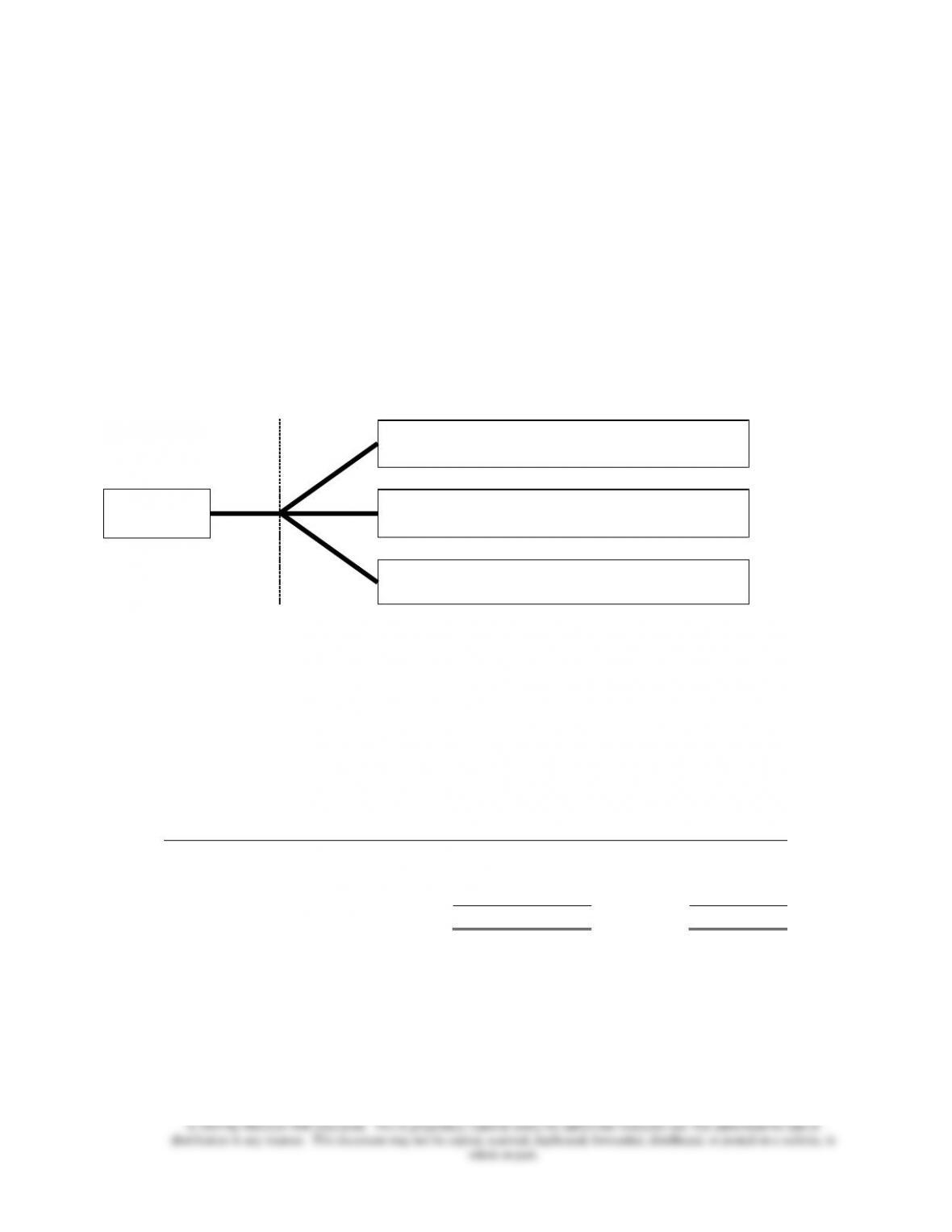
Superior Refinery produces oil products in a joint production process. For the month of October,
$450,000 of materials, labor, and overhead were added to produce the three main products: M1,
M2, and M3. The sale values were available right after the split-off point. The following diagram
shows the process.
M1
Sale value $200,000
Joint costs
$450,000
M2
Sale value $300,000
M3
Sale value $500,000

Chapter 11 – Service Department and Joint Cost Allocation
11–16
Required:
Allocate the joint costs to the products using the net realizable value method.
Solution:
The cost allocation follows the proportional distribution of net realizable values.
Product
Sale value
Proportion
Allocation
M1
$200,000
20%a
$90,000b
M2
300,000
30%
135,000
M3
500,000
50%
225,000
Total
$1,000,000
$450,000
a 20% = $200,000 ÷ $1,000,000.
b $90,000 = $450,000 × 20%.
======================
• If the products require further processing before they are marketable, it may be
necessary to estimate the net realizable value at the split-off point using the estimated
net realizable value method (sometimes called the netback or workback method).
Estimated
net realizable
value
=
Sales price of a
final product after
further processing
–
Additional processing costs
necessary to prepare a
product for sale
• Under the net realizable value method, revenue dollars from any joint product are
assumed to make the same percentage contribution at the split-off point as the revenue
dollars from any other joint product. That is, each joint product gets the same gross
margin percentage.
Example 2: For Demonstration Problem 5 above, the gross margin for all the joint
products can be calculated as follows.
M1
M2
M3
Total
Sales
$200,000
$300,000
$500,000
$1,000,000
Allocated joint costs
90,000
135,000
225,000
450,000
Gross margin
$110,000
$165,000
$275,000
$550,000
Gross margin percentage
55%
55%
55%
55%
The gross margin percentage is the same for all the joint products when the net
realizable value method is used.
Chapter 11 – Service Department and Joint Cost Allocation
11–17
• The net realizable value method implies a matching of input costs with revenues
generated by each output.
======================
Demonstration Problem 6
(Continued from Demonstration Problem 5)
Products M1 and M2 needed further processing with additional costs before they could be
marketable. Product M3 was immediately available for sale. The following diagram shows the
process.
M1
Processing cost $120,000, Sale value $300,000
Joint costs
$450,000
M2
Processing cost $80,000, Sale value $400,000
M3
Sale value $500,000
Required:
Allocate the joint costs to the products using the estimated net realizable value method.
Solution:
The estimated net realizable value is used for joint cost allocation in the same way as an
actual market value at the split-off point.
a 18% = $180,000 ÷ $1,000,000.
b $81,000 = $450,000 × 18%.
======================
Product
Sale value
(1)
Processing
cost
(2)
Estimated net
realizable value
(1) – (2)
Proportion
Allocation
M1
$300,000
$120,000
$180,000
18%a
$81,000b
M2
400,000
80,000
320,000
32%
144,000
M3
500,000
0
500,000
50%
225,000
Total
$1,000,000
$450,000

Chapter 11 – Service Department and Joint Cost Allocation
11–18
LO 11-8 Allocate joint costs using the physical quantities method.
♦ Physical quantities method allocates joint costs based on measurement of the volume, weight,
or other physical measure of the joint products at the split-off point.
• The physical quantities method is used when
(1) output product prices are highly volatile,
(2) significant processing occurs between the split-off point and the first point of
marketability, or
(3) product prices are not set by the market.
• Many companies allocate joint costs incurred in producing oil and gas on the basis of
energy equivalent (BTU content).
======================
Demonstration Problem 7
(Continued from Demonstration Problem 5)
Superior Refinery produces oil products in a joint production process. For the month of October,
$450,000 of materials, labor and overhead were added to produce the three main products: M1,
M2, and M3. The physical quantities of the outputs are considered relevant for cost allocation
purposes. The following diagram shows the process.
M1
15,000 units
Joint costs
$450,000
M2
20,000 units
M3
25,000 units
Required:
Allocate the joint costs to the products using the physical quantities method.

Chapter 11 – Service Department and Joint Cost Allocation
11–19
Solution:
The allocation of joint costs is based on the physical units in this case.
Product
Units
Proportion
Allocation
M1
15,000
25.0%a
$112,500b
M2
20,000
33.3%
150,000
M3
25,000
41.7%
187,500
Total
60,000
$450,000
a 25% = 15,000 ÷ 60,000.
b $112,500 = $450,000 × 25%.
======================
♦ The “jointness” of the joint production process makes it impossible to separate the portion of
joint costs attributable to one product from another on a cause-and-effect basis.
• Accountants and managers realize that no one allocation method is appropriate for all
situations.
• If allocated joint costs are used for decision-making purposes, they should be used only
with full recognition of their limitations.
LO 11-9 Explain how cost data are used in the sell-or-process-further
decision.
♦ Managers must decide whether it is more profitable to sell the output at an intermediate stage
or to process it further.
• The relevant data to be considered are
(1) the additional revenue after further processing, and
(2) the additional costs of processing further.
• The decision rules about whether to process further are as follows.
Sell at split-off point if: Sales value at split-off > (Sales value after process – Additional
processing cost)
Process further if: Sales value at split off < (Sales value after process – Additional
processing cost)