Unlock document.
This document is partially blurred.
Unlock all pages and 1 million more documents.
Get Access
Chapter 10S - Acceptance Sampling
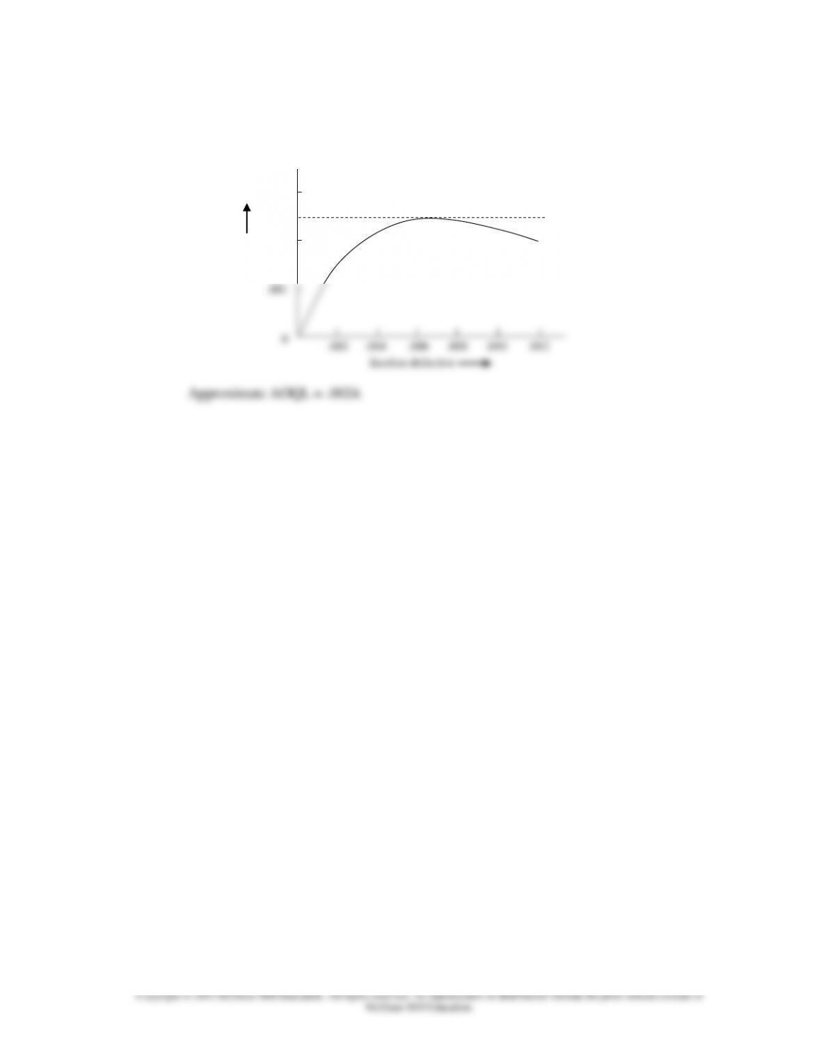
c. AOQ Curve and AOQL for data in part b:
OC Curve
AOQ
c.
.003
.002
AOQL .0024
Chapter 10S - Acceptance Sampling
4. Given:
N = 3,000
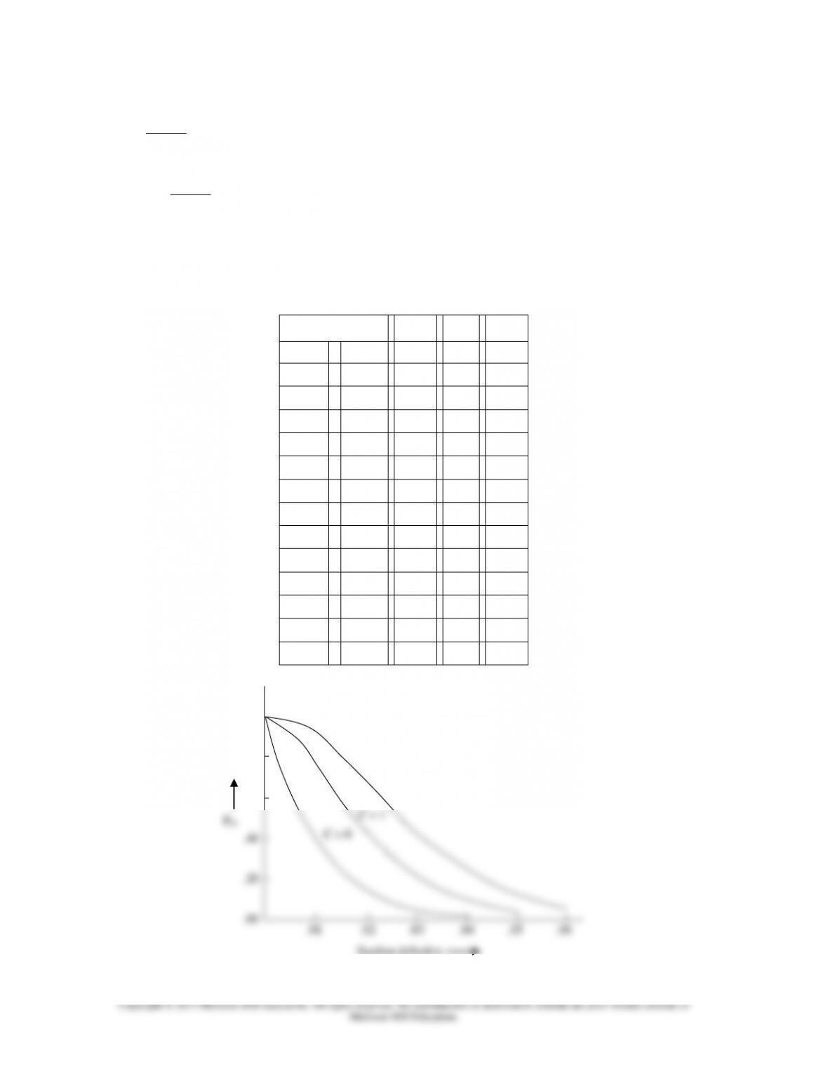
a. Given:
n = 100
c = 0, 1, & 2.
Use the Poisson distribution table from Appendix B because n > 20 & p < .05 as
shown in the table below.
[n = 100]
c = 0
c = 1
c = 2
p
μ = np
Pac
Pac
Pac
.001
.1
.905
.995
1.000
.002
.2
.819
.982
.999
.003
.3
.741
.963
.996
.004
.4
.670
.938
.992
.005
.5
.607
.910
.986
.006
.6
.549
.878
.977
.008
.8
.449
.809
.953
.010
1.0
.368
.736
.920
.015
1.5
.223
.558
.809
.020
2.0
.135
.406
.677
.030
3.0
.050
.199
.423
.040
4.0
.018
.092
.238
.050
5.0
.007
.040
.125
C = 2
1.00
.80
.60
fraction defective
OC Curves
Chapter 10S - Acceptance Sampling
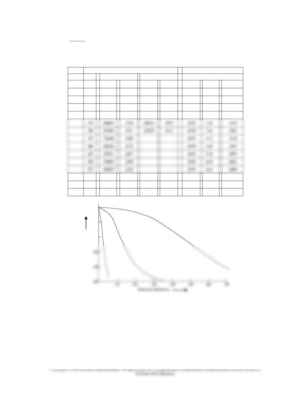
b. Given:
c = 2; n = 5, 20, & 120:
Note: We can use the binomial distribution table for the first two values of n, but we must
use the Poisson distribution table for the third value of n = 120.
[Binomial table]
[Poisson table]
n = 5
n = 20
n = 120
c = 2
p
Pac
AOQ
Pac
AOQ
p
μ = np
Pac
.05
.9988
.050
.9245
.046
.005
.6
.977
.10
.9914
.099
.6769
.068
.010
1.2
.880
.15
.9734
.146
.4049
.061
.015
1.8
.731
.20
.9421
.188
.2061
.041
.020
2.4
.570
.25
.8965
.224
.0913
.023
.025
3.0
.423
.30
.8369
.251
.0355
.011
.030
3.6
.303
.35
.7648
.268
.035
4.2
.210
.40
.6826
.273
.040
4.8
.143
.45
.5931
.267
.045
5.4
.095
.50
.5000
.250
.050
6.0
.062
.55
.4069
.224
.055
6.6
.040
.60
.3174
.190
.65
.2352
.153
.70
.1631
.114
n = 5
n = 20
n = 120
1.00
.80
.60
fraction defective
Pac
OC Curves
10S-10
5. Given:
Samples of n = 15 parts are inspected. Inspection cost = $1/unit. Replacement cost =
$6.25/unit. Shipments of several thousand parts per week are received from a supplier.
a. Fraction defective at which the manufacturer would be indifferent between 100%
inspection and replacement:
x = $1/$6.25
x = .1600 (round to a maximum of four decimals)
b. Maximum number of sample defectives that would cause the lot to be passed without
100% inspection based on part a:
Expected Number of Defectives = Fraction Defective * Number in Sample
(2) Probability that the shipment would be rejected in favor of 100% inspection:
Using the binomial distribution table from Appendix B with n = 15, c = x = 2, & p =
.05:
Pac = .9638
Chapter 10S - Acceptance Sampling
10S-11
(4) The producer’s risk occurs when a shipment (lot) that satisfies the standard is rejected.
If the shipment contains 5% defective, the correct decision is to accept it (the standard
is 16%). Even so, there is a risk that a sample will contain more than 2 defective and
that the shipment would be rejected:
shipment has only 5% defective, it satisfies the standard. Therefore, accept is the
correct decision, and the consumer’s risk is zero. In other words, there is zero
probability that the shipment will have more than the standard (specified percentage
of defective items).
d. Shipment actually contains 20% defective items:
(1) If the percentage defective = 20%, reject because percentage defective > 16%.
(3) Probability that the shipment would be accepted without 100% inspection = Pac =
(4) The producer’s risk occurs when a shipment (lot) that satisfies the standard is rejected.
If the shipment contains 20% defective, the correct decision is to reject the shipment
because the shipment does not meet the standard (16%). There is zero producer’s
risk of a good shipment being rejected because the shipment is not good, i.e. it does
not satisfy the standard.
The consumer’s risk occurs when a shipment (lot) is accepted that has more than the
standard (specified percentage of defective items). Here that percentage is 16%. If the
10S-12
6. Given:
Refer back to Problem 5 part c. There are two defectives in the sample.
a. Given:
Acceptance number = c = 1
Reject lot because 2 > 1.
A Type I error (producer’s risk) is possible, i.e., rejecting a lot containing the acceptable
quality level.
b. Given:
Acceptance number = c = 3
Accept lot because 2 ≤ 3.
A Type II error (consumer’s risk) is possible, i.e., accepting a bad lot based on an analysis
of the sample data.
c. Use the binomial distribution table from Appendix B with n = 15 & c = x = 1 (round all
values to four decimals):
(1) .05(.8290) = .0415


