Chapter 08S – The Transportation Model
CHAPTER 08S
THE TRANSPORTATION MODEL
Teaching Notes
The transportation method seems to be middle-of-the-road in terms of students’ abilities to develop an
intuitive feel for what is happening during the process. Although in practice much of the actual
computations are done by computers using the simplex algorithm, I feel that students gain a certain
amount of insight and intuitive understanding by going through the calculations.
Cell evaluations are illustrated using the stepping-stone method and the MODI method. While it may
be more efficient to use the MODI method, note that for the size of the problems students will
encounter, the two methods are probably similar in terms of efficiency. Consequently, I think it is
more a matter of personal preference regarding which method is used.
Answers to Discussion and Review Questions
1. To use the transportation model we need the following:
2. Before proceeding to develop an initial solution, we must check to see that supply and demand
3. It would never make sense to have a situation that required both a dummy row and a dummy
column. A dummy is added to supply or demand, whichever is lower.
4. Transportation costs per unit are treated as a direct linear function of the number of units
shipped in the objective function.
5. The + and – signs alternate in cell evaluation paths to maintain the row and the column totals
given.
6. A solution is optimum when there are no empty cells with negative cell evaluations.
7. A zero value for an evaluation path indicates no impact whatsoever on transportation costs,
8. If a solution is not optimal:
a. We shift units into the empty cell with the largest negative cell evaluation.
9. Degeneracy exists when there are too few completed cells to allow all necessary paths to be
constructed.
8S-2
10. The transportation model can be used to compare location alternatives in terms of their impact
on the total distribution costs for a system. The procedure involves working through a separate
11. Totals costs for a given distribution plan are determined by summing the following over all
cells: units shipped in each cell multiplied by unit shipping cost.
12. Units allocated to a dummy destination are not actually shipped to the dummy destination.
This is a fictitious number that represents the amount by which total supply exceeds total
13. The modified distribution method (MODI) is a method for evaluating empty cells. It involves
computing row and column index numbers that can be used for cell evaluation.
Chapter 08S – The Transportation Model
Solutions to Problems
1. Solve this problem using the transportation method. Find the optimal transportation plan and
the minimum cost. Also, decide if there is an alternate solution. If there is one, identify it.
Given:
From:
To:
1
2
3
Supply
8
2
5
1
90
2
1
3
2
105
7
2
6
3
105
Demand
150
75
75
300 \ 300
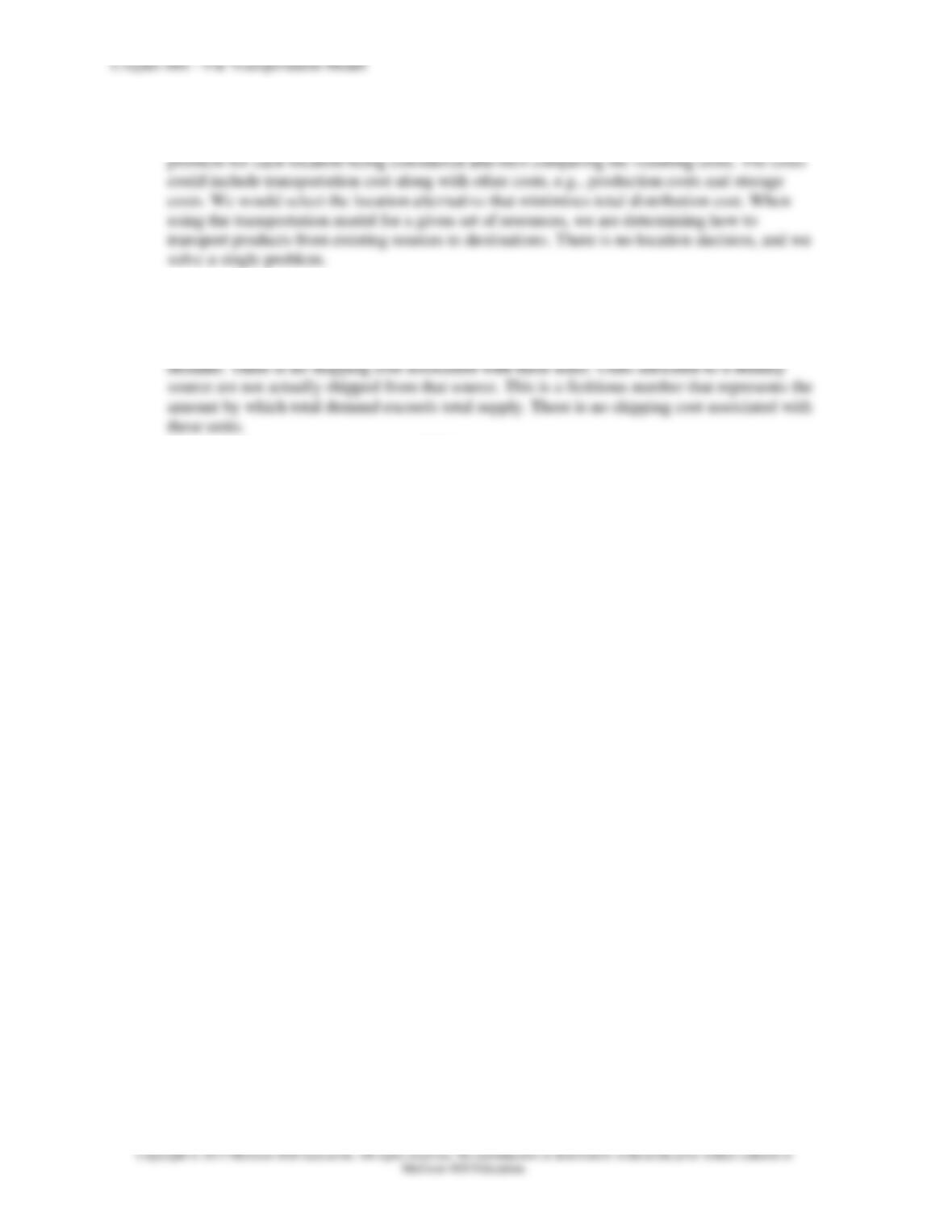
Step 1: Initial Solution with Intuitive Lowest-Cost Approach:
(a) Check to see if supply and demand are equal. They are equal—no dummy is necessary.
(b) Find the cell in the table above that has the lowest unit transportation cost. Cell 2-2 has the
lowest cost ($1). Assign as many units as possible to this cell: minimum of 105 & 75 = 75.
This exhausts the Column 2 total, so cross out 75, and cross out the cell costs for Column
2. Revise the Row 2 total to 30. The result is shown below.
From:
To:
1
2
3
Supply
8
2
5
1
90
2
1
3
2
75
105 30
7
2
6
3
105
Demand
150
75
75
300 \ 300
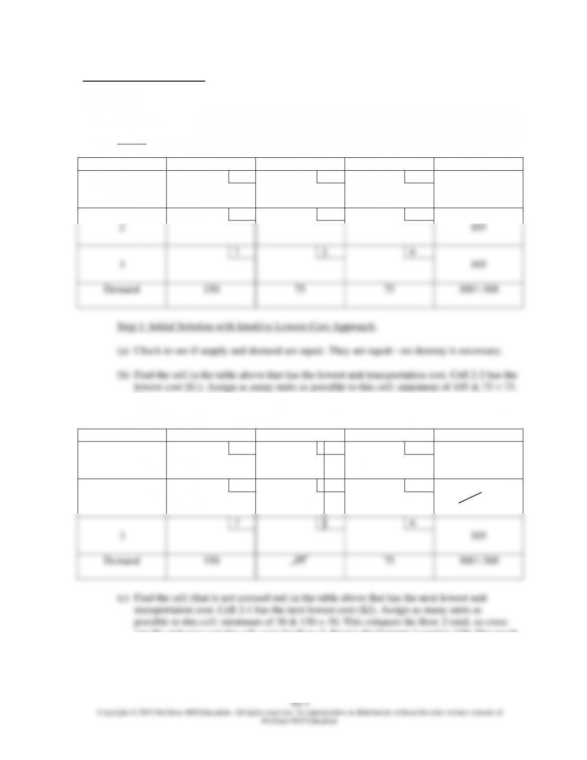
(c) Find the cell (that is not crossed out) in the table above that has the next lowest unit
transportation cost. Cell 2-1 has the next lowest cost ($2). Assign as many units as
possible to this cell: minimum of 30 & 150 = 30. This exhausts the Row 2 total, so cross
out 30, and cross out the cell costs for Row 2. Revise the Column 1 total to 120. The result
is shown below.
Chapter 08S – The Transportation Model
From:
To:
1
2
3
Supply
8
2
5
1
90
2
1
3
2
30
75
105 30
7
2
6
3
105
Demand
150 120
75
75
300 \ 300
(d) Find the cell (that is not crossed out) in the table above that has the next lowest unit
transportation cost. Cell 1-3 has the next lowest cost ($5). Assign as many units as
possible to this cell: minimum of 90 & 75 = 75. This exhausts the Column 3 total, so cross
out 75, and cross out the cell costs for Column 3. Revise the Row 1 total to 15. The result
is shown below.
From:
To:
1
2
3
Supply
8
2
5
1
75
90 15
2
1
3
2
30
75
105 30
7
2
6
3
105
Demand
150 120
75
75
300 \ 300
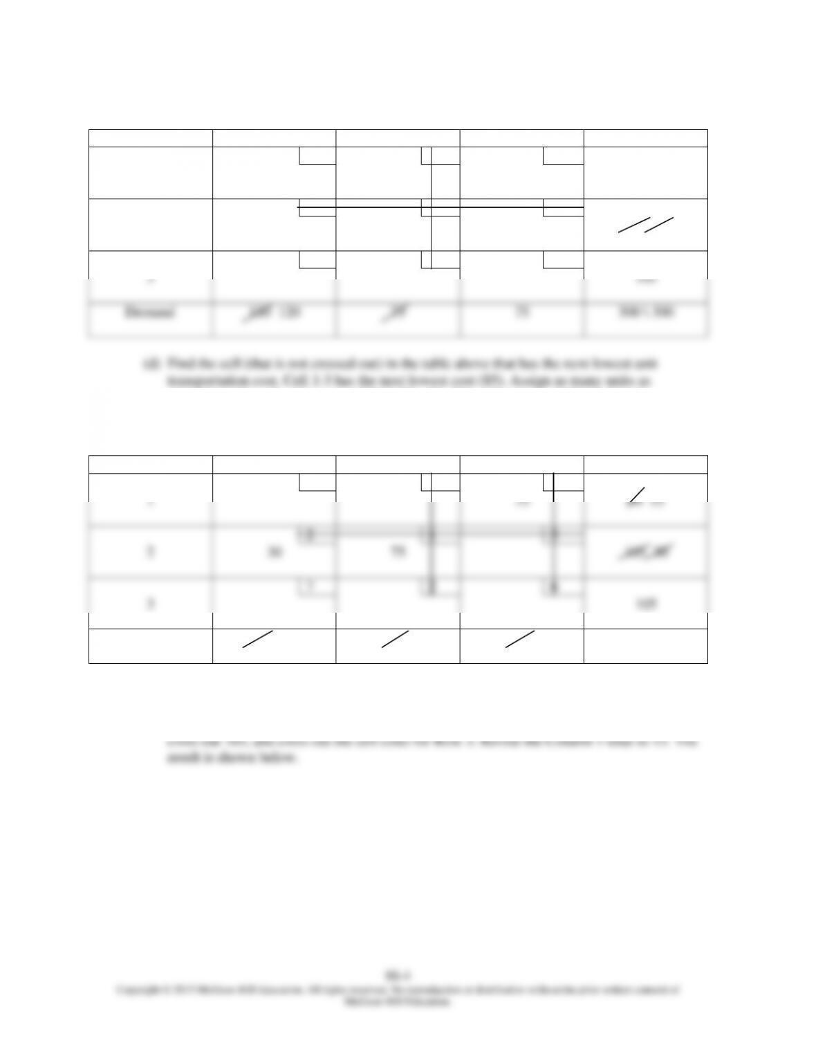
(e) Find the cell (that is not crossed out) in the table above that has the next lowest unit
transportation cost. Cell 3-1 has the next lowest cost ($7). Assign as many units as
possible to this cell: minimum of 105 & 120 = 105. This exhausts the Row 3 total, so
Chapter 08S – The Transportation Model
8S-5
From:
To:
1
2
3
Supply
8
2
5
1
75
90 15
2
1
3
2
30
75
105 30
7
2
6
3
105
105
Demand
150 120 15
75
75
300 \ 300
(f) Find the cell (that is not crossed out) in the table above that has the next lowest unit
transportation cost. Cell 1-1 has the next lowest cost ($8). Assign as many units as
possible to this cell: minimum of 15 & 15 = 15. This exhausts the Row 1 and Column 1
totals. The initial solution is shown below.
From:
To:
1
2
3
Supply
8
2
5
1
15
75
90
2
1
3
2
30
75
105
7
2
6
3
105
105
Demand
150
75
75
300 \ 300
Total cost = (15 x 8) + (75 x 5) + (30 x 2) + (75 x 1) + (105 x 7) = $1,365.
Step 2: Evaluate empty cells with the MODI method:
Chapter 08S – The Transportation Model
(b) Obtain an index number of each row and column. Do this using only occupied cells. Index
Chapter 08S – The Transportation Model
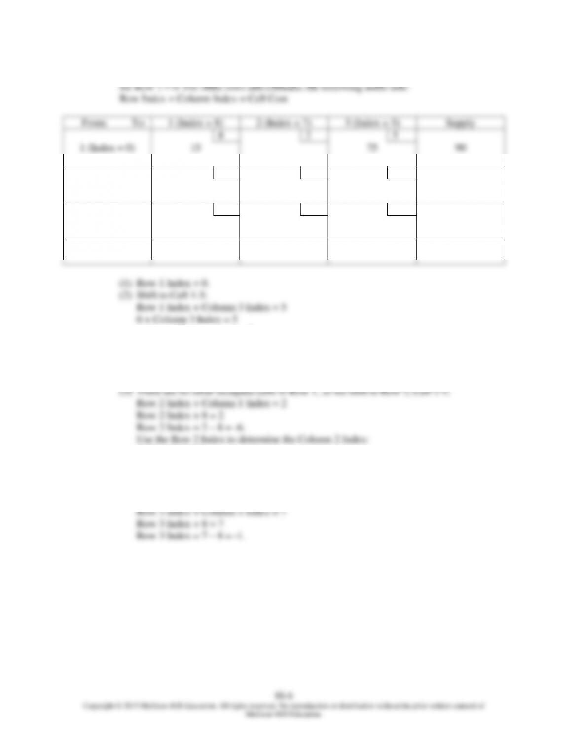
(c) Evaluate the empty cells using the following formula:
Cell Evaluation = Cell Cost – (Row Index + Column Index)
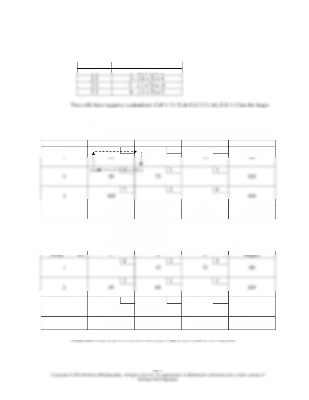
Cell
Evaluation
1-2
2 – (0 + 7) = –5
2-3
3 – (-6 + 5) = 4
3-2
2 – (-1 + 7) = –4
3-3
6 – (-1 + 5) = 2
Two cells have negative evaluations: Cell 1-2 (-5) & Cell 3-2 (-4). Cell 1-2 has the larger
negative value, so we shift as many units as possible to Cell 1-2. The stepping stone path
for Cell 1-2 is shown below.
Cell 1-2 Stepping Stone Path
From:
To:
1
2
3
Supply
(-)
8
(+)
2
5
1
15
75
90
(+)
2
(-)
1
3
2
30
75
105
7
2
6
3
105
105
Demand
150
75
75
300 \ 300
The quantities in the cells that have – signs are potential candidates for shifting units. Cell
2-2 has 75 units and Cell 1-1 has 15 units. Therefore, 15 units can be shifted. The result is
shown below.
From:
To:
1
2
3
Supply
8
2
5
1
15
75
90
2
1
3
2
45
60
105
7
2
6
3
105
105
Demand
150
75
75
300 \ 300
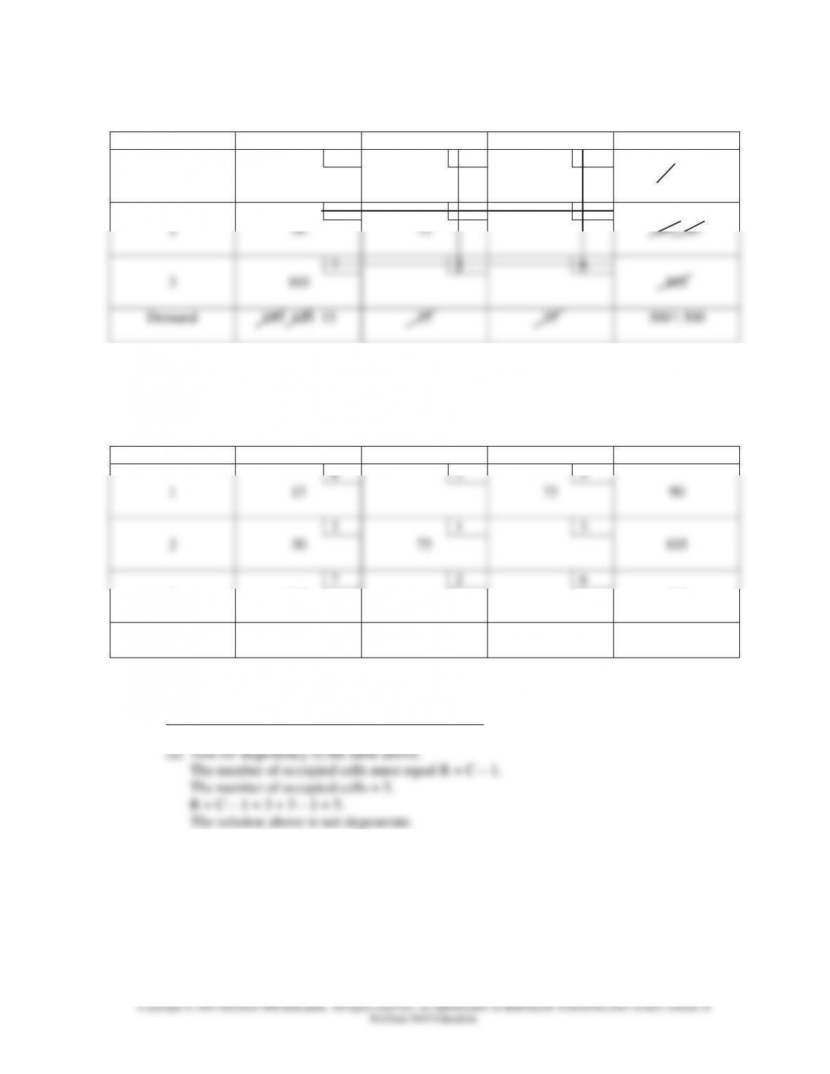
The number of occupied cells must equal R + C – 1.
The number of occupied cells = 5.
R + C – 1 = 3 + 3 – 1 = 5.
The solution above is not degenerate.
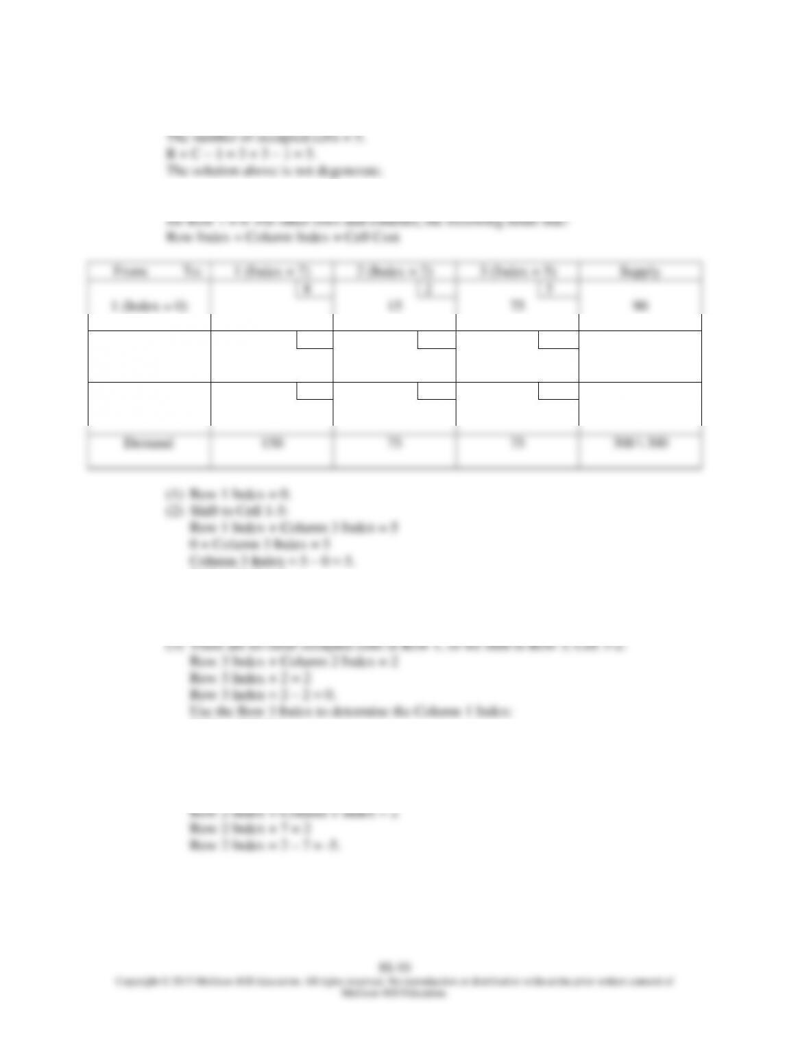
(e) Obtain an index number of each row and column. Do this using only occupied cells. Index
Chapter 08S – The Transportation Model
(f) Evaluate the empty cells using the following formula:
Cell Evaluation = Cell Cost – (Row Index + Column Index)
Cell
Evaluation
1-1
8 – (0 + 3) = 5
2-3
3 – (-1 + 5) = –1
3-2
2 – (4 +2) = –4
3-3
6 – (4 + 5) = –3
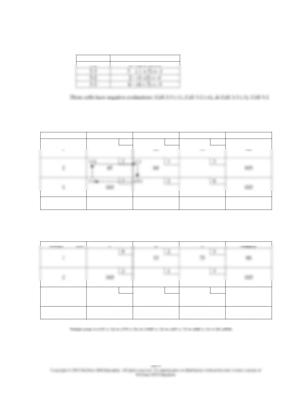
Three cells have negative evaluations: Cell 2-3 (-1), Cell 3-2 (-4), & Cell 3-3 (-3). Cell 3-2
has the largest negative value, so we shift as many units as possible to Cell 3-2. The
stepping stone path for Cell 3-2 is shown below.
Cell 3-2 Stepping Stone Path
From:
To:
1
2
3
Supply
8
2
5
1
15
75
90
(+)
2
(-)
1
3
2
45
60
105
(-)
7
(+)
2
6
3
105
105
Demand
150
75
75
300 \ 300
The quantities in the cells that have – signs are potential candidates for shifting units. Cell
2-2 has 60 units and Cell 3-1 has 105 units. Therefore, 60 units can be shifted. The result
is shown below.
From:
To:
1
2
3
Supply
8
2
5
1
15
75
90
2
1
3
2
105
105
7
2
6
3
45
60
105
Demand
150
75
75
300 \ 300
Total cost = (15 x 2) + (75 x 5) + (105 x 2) + (45 x 7) + (60 x 2) = $1,050.
Chapter 08S – The Transportation Model
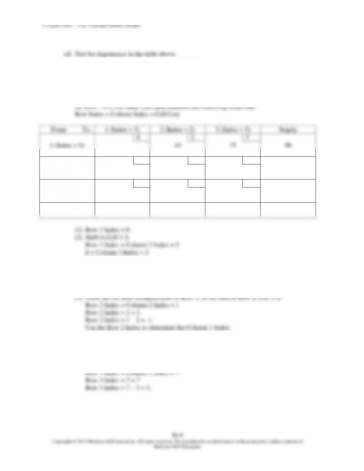
(g) Test for degeneracy in the table above.
The number of occupied cells must equal R + C – 1.
(h) Obtain an index number of each row and column. Do this using only occupied cells. Index