Chapter 05S – Decision Theory
5S–21
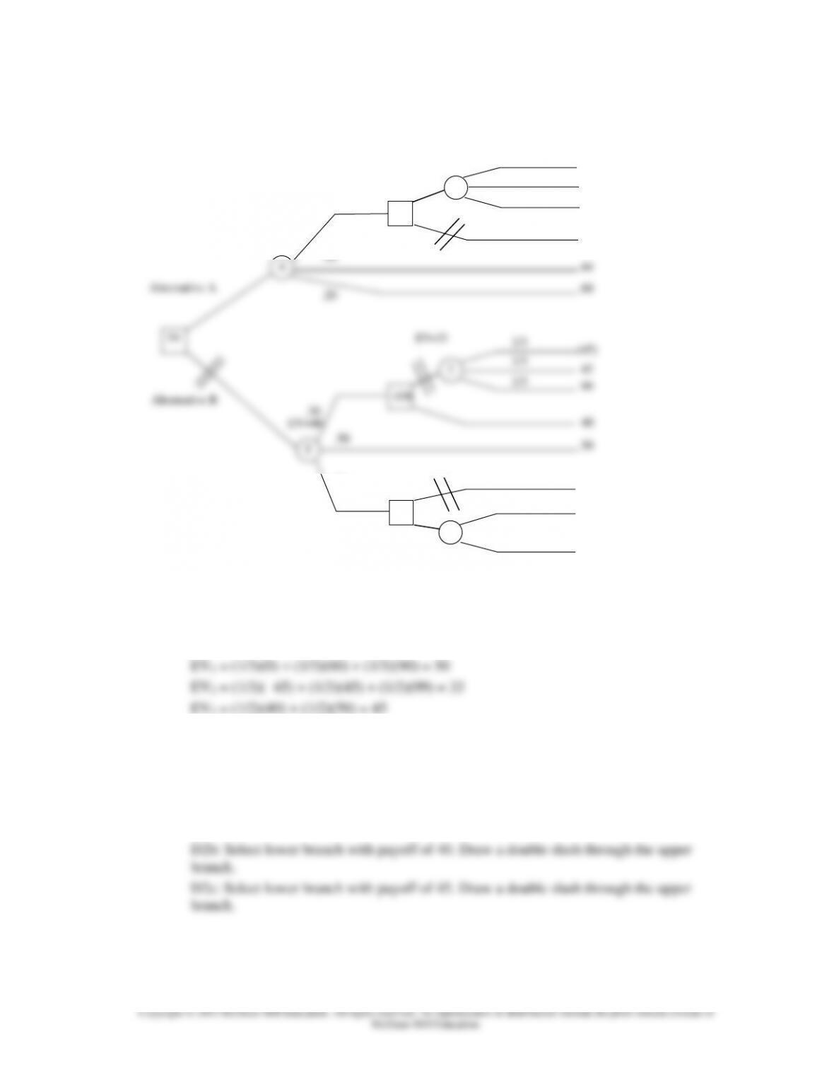
11. Decision Tree
Alternative A
.20
60
D2b
1/3
50
5
44
40
4
EV=46
1) Determine the product of the chance probabilities and their respective payoffs for the
branches on the right hand side. Because this is a complex problem, we have added labels
to the circles:
2) Determine which alternative would be selected for each possible second decision. We
have labeled these D2a, D2b, and D2c.
D2a: Select upper branch with payoff of 50. Draw a double slash through the lower
branch.
.30
.50
60
40
D2a
0
90
1
1/3
D2c
.20
3
50
1/2
1/3
1/3
30
1/2
40
EV=49
EV=50
EV=45
Chapter 05S – Decision Theory
5S–22
3) Determine the product of the chance probabilities and their respective payoffs for the
branches on the left hand side. Because this is a complex problem, we have added labels
to the circles:
4) Determine the expected value of each initial alternative.
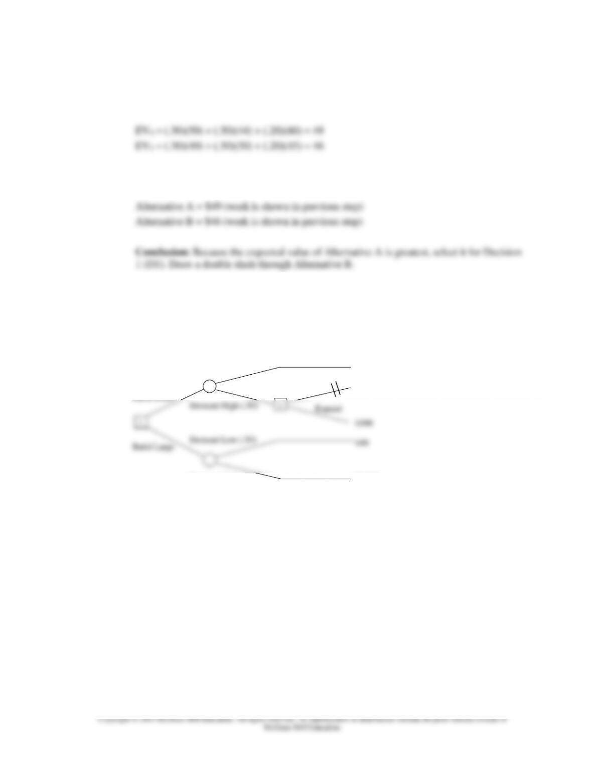
12. a.
1) Draw the tree diagram. Because the probabilities are unknown, we would assume that
each state of nature has an equal probability of occurring.
2) We have to make a choice for the possible second decision before proceeding.
Expand has a higher payoff than Lease ($500 > $100). Select Expand. Draw a double
slash through the Lease branch.
$700
$100
$500
$40
$2,000
Demand Low (.50)
Demand Low (.50)
Demand High (.50)
Demand High (.50)
Lease
Expand
Build Small
Build Large
1
2
5S–23
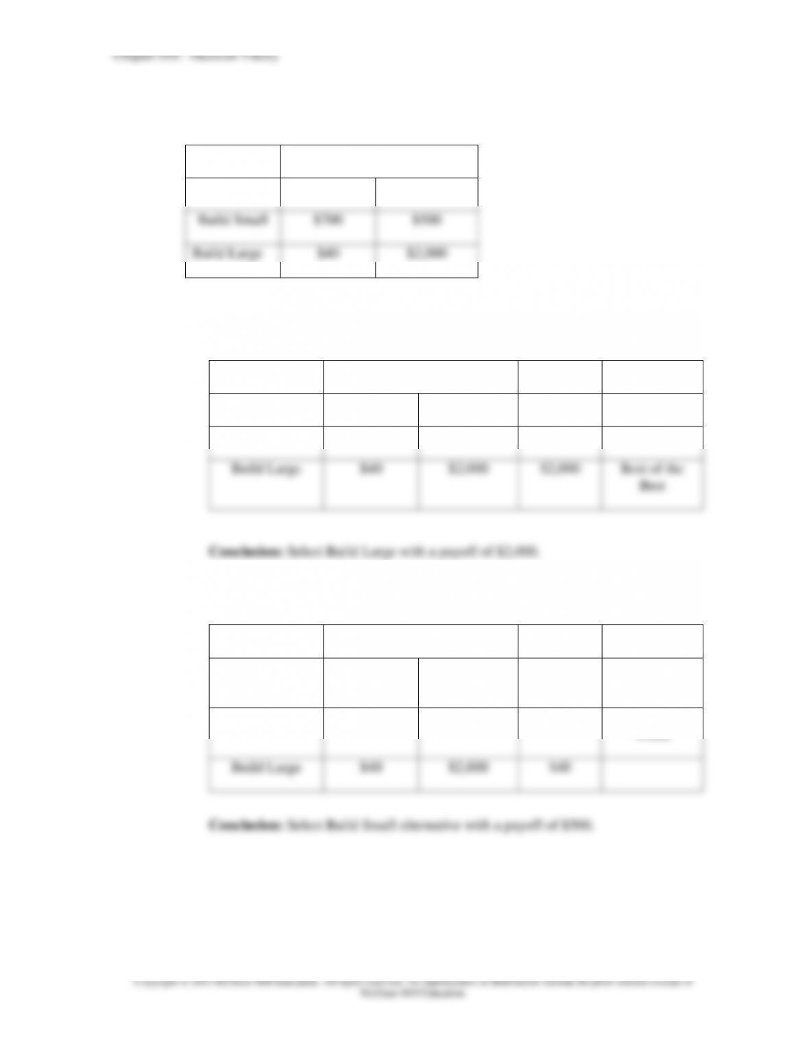
b. Use the tree diagram to identify the choice that you would make using each of the four
approaches for decision making under uncertainty.
States of Nature
Alternative
Demand Low
Demand High
Build Small
$700
$500
Build Large
$40
$2,000
1) Maximax: Determine best possible payoff for each alternative and choose the
alternative that has the “best.”
States of Nature
Alternative
Demand Low
Demand High
Best Payoff
Build Small
$700
$500
$700
Build Large
$40
$2,000
$2,000
Best of the
Best
Conclusion: Select Build Large with a payoff of $2,000.
2) Maximin: Determine the worst possible payoff for each alternative and choose the
alternative that has the “best worst.”
States of Nature
Alternative
Demand Low
Demand High
Worst
Payoff
Build Small
$700
$500
$500
Best of the
Worst
Build Large
$40
$2,000
$40
Conclusion: Select Build Small alternative with a payoff of $500.
Chapter 05S – Decision Theory
5S–24
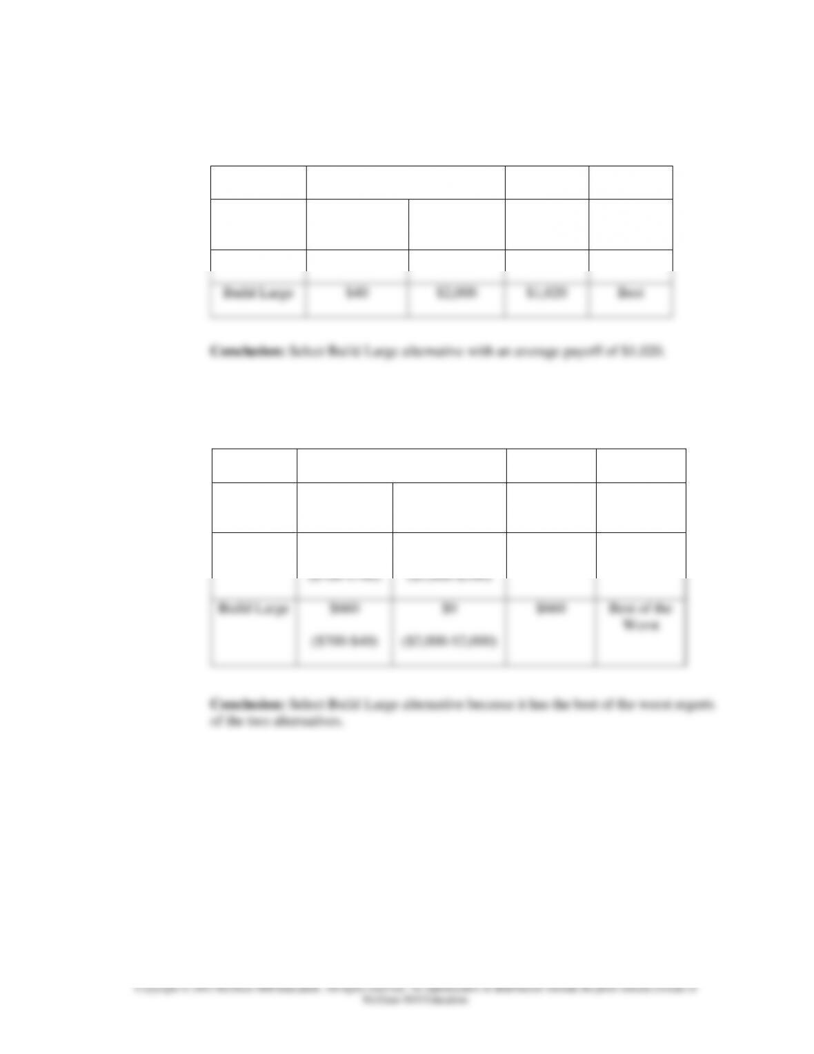
3) Laplace: Determine the average payoff for each alternative and choose the alternative
with the best average.
States of Nature
Alternative
Demand Low
Demand High
Average
Payoff
Build Small
$700
$500
$600
Build Large
$40
$2,000
$1,020
Best
Conclusion: Select Build Large alternative with an average payoff of $1,020.
4) Minimax Regret: Prepare a table of regrets (opportunity losses)—for each column,
subtract every payoff from the best payoff in that column. Identify the worst regret for
each alternative. Select the alternative with the “best worst.”
Build Large
($700-$40)
Regrets
Alternative
Demand Low
Demand High
Worst
Regret
Build Small
$0
($700-$700)
$1,500
($2,000-$500)
$1,500
Chapter 05S – Decision Theory
5S–25
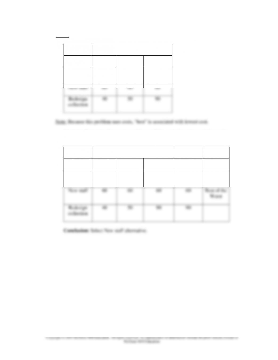
13. Given: We have the estimated costs for various alternatives and caseloads shown below.
Caseload
Alternative
Moderate
High
Very High
Reassign
staff
50
60
85
New staff
60
60
60
Redesign
collection
40
50
90
alternative that has the “best worst.”
Caseload
Alternative
Moderate
High
Very High
Worst
Reassign
staff
50
60
85
85
New staff
60
60
60
60
Best of the
Worst
Redesign
collection
40
50
90
90
Conclusion: Select New staff alternative.
Chapter 05S – Decision Theory
5S–26
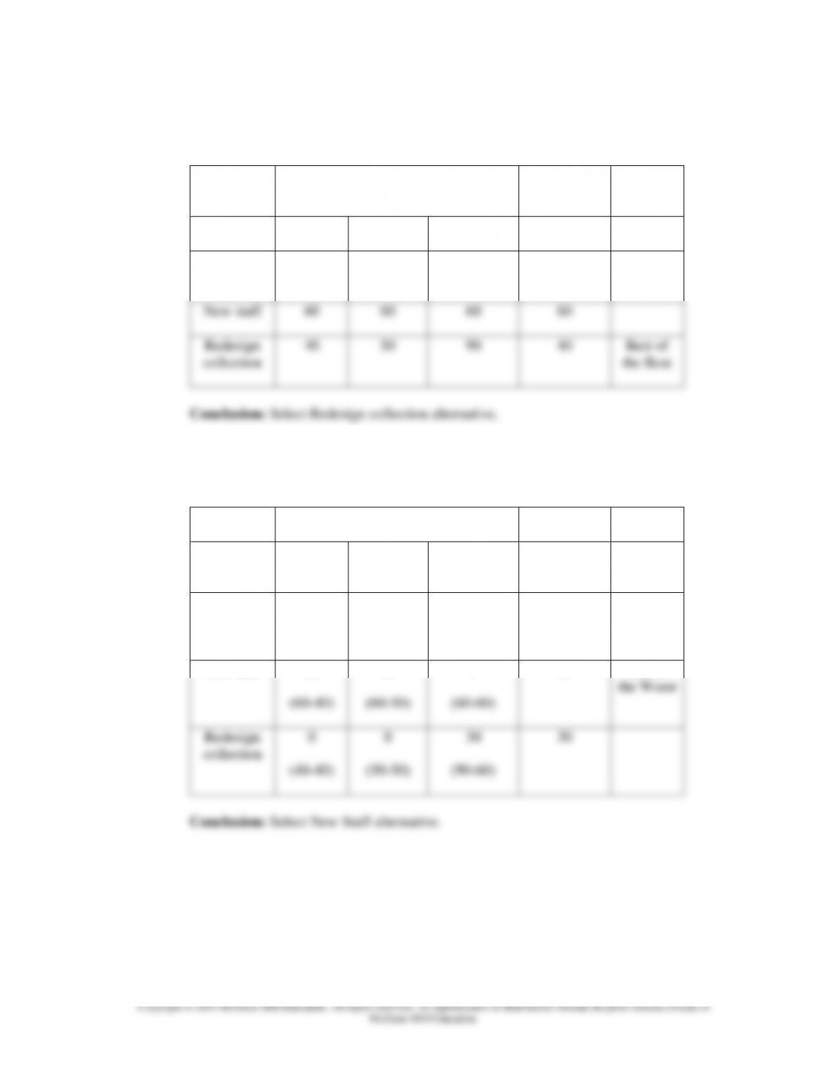
b. Maximax: Determine best possible payoff for each alternative and choose the alternative
that has the “best.”
Caseload
Alternative
Moderate
High
Very High
Best
Reassign
staff
50
60
85
50
New staff
60
60
60
60
Redesign
collection
40
50
90
40
Best of
the Best
Conclusion: Select Redesign collection alternative.
c. Minimax Regret: Prepare a table of regrets (opportunity losses)—for each column,
subtract every payoff from the best payoff in that column. Identify the worst regret for
each alternative. Select the alternative with the “best worst.”
Regret
Alternative
Moderate
High
Very High
Worst
Regret
Reassign
staff
10
(50-40)
10
(60-50)
25
(85-60)
25
New staff
20
(60-40)
10
(60-50)
0
(60-60)
20
Best of
the Worst
Redesign
collection
0
(40-40)
0
(50-50)
30
(90-60)
30
Conclusion: Select New Staff alternative.
Chapter 05S – Decision Theory
5S–27
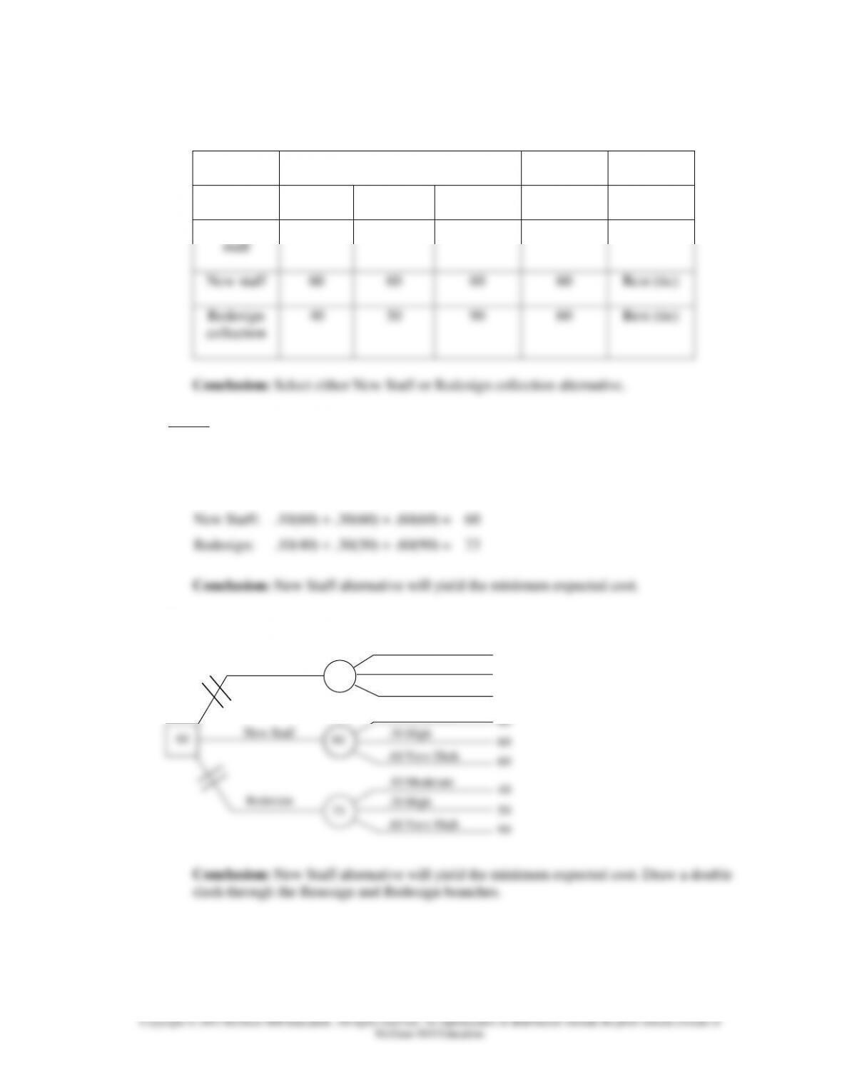
d. Laplace: Determine the average payoff for each alternative and choose the alternative with
the best average.
Caseload
Alternative
Moderate
High
Very High
Average
Reassign
staff
50
60
85
65
New staff
60
60
60
60
Best (tie)
Redesign
collection
40
50
90
60
Best (tie)
Conclusion: Select either New Staff or Redesign collection alternative.
14. Given: Probabilities for states of nature are now given as follows: .10 for moderate, .30 for
high, and .60 for very high.
a. Minimum expected cost:
Reassign:
.10(50) + .30(60) + .60(85) =
$74
New Staff:
.10(60) + .30(60) + .60(60) =
60
Redesign:
.10(40) + .30(50) + .60(90) =
73
Conclusion: New Staff alternative will yield the minimum expected cost.
b.
New Staff
Reassign
Redesign
50
60
85
60
60
60
40
50
90
.30 High
.60 Very High
.10 Moderate
.30 High
.60 Very High
.10 Moderate
.30 High
.60 Very High
.10 Moderate
74
60
73
60
Chapter 05S – Decision Theory
5S–28
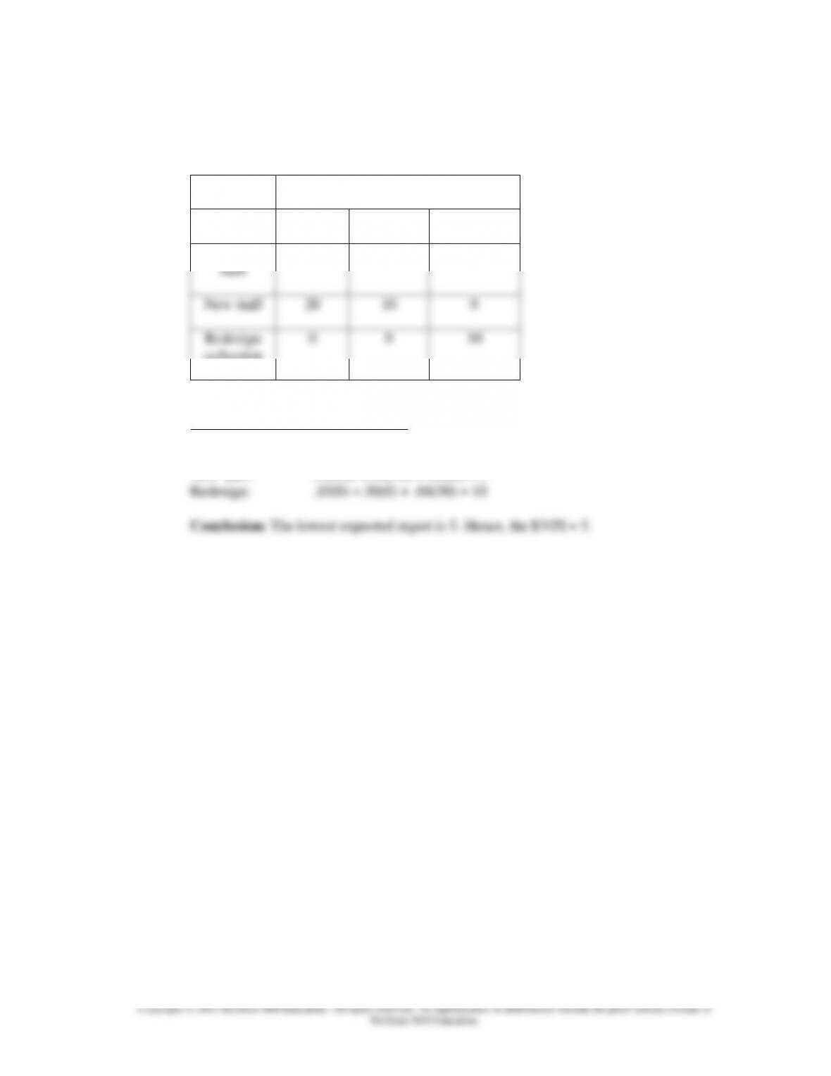
c. Opportunity loss table
Regret
Alternative
Moderate
High
Very High
Reassign
staff
10
10
25
New staff
20
10
0
Redesign
collection
0
0
30
Expected regret for each alternative:
Reassign: .10(10) +.30(10) + .60(25) = 19
New staff: .10(20) +.30(10) + .60(0) = 5
Chapter 05S – Decision Theory
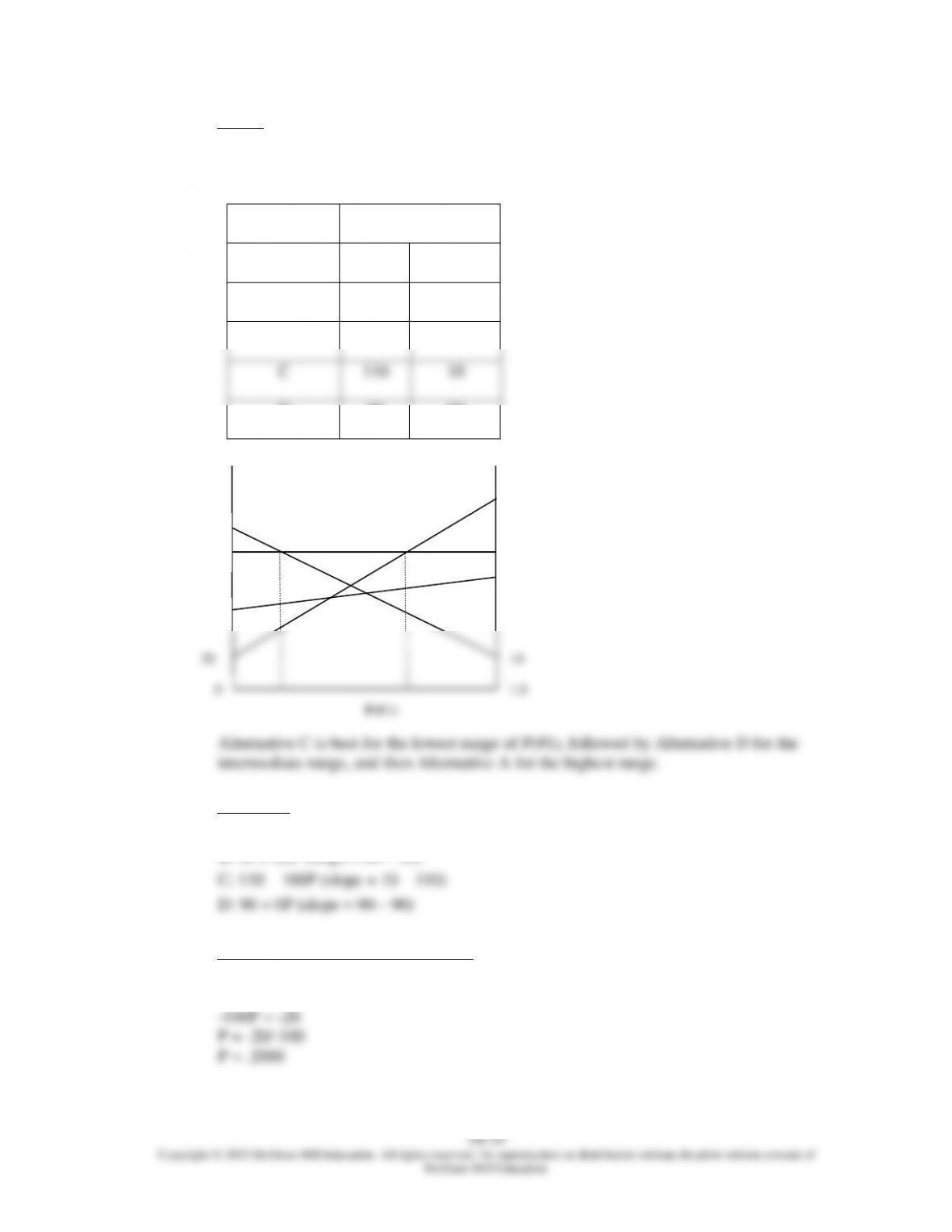
15. a. Given: Payoffs (profits) are provided in the table below.
Plot each alternative relative to P(1). Plot the payoff value for #2 on the left side of the
graph and the payoff value for #1 on the right side of the graph.
State of Nature
Alternative
#2
#1
A
20
120
B
40
60
C
110
10
D
90
90
10
Equations:
A: 20 + 100P (slope = 120 – 20)
B: 40 + 20P (slope = 60 – 40)
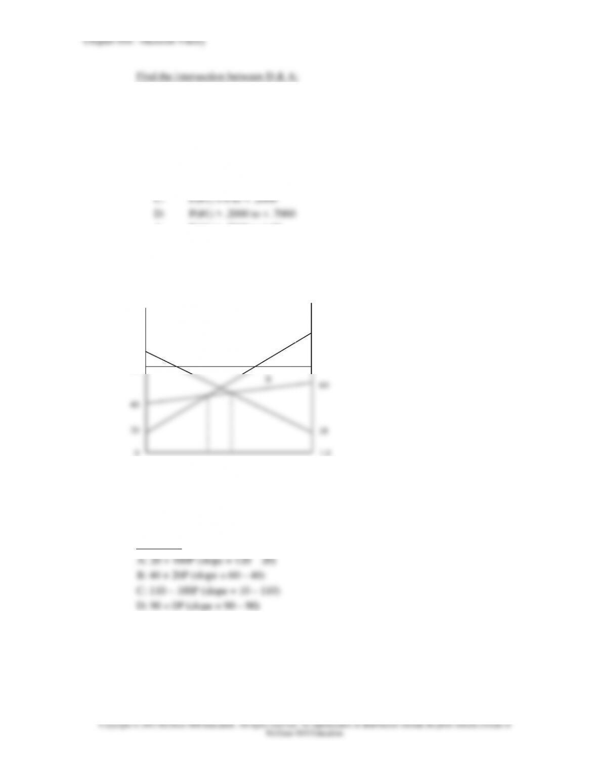
Find the intersection between C & D:
110 – 100P = 90 + 0P
-100P = 90 – 110
C
110
90
B
#2
#1
120
A
D
40
90
60
5S–30
Copyright © 2015 McGraw-Hill Education. All rights reserved. No reproduction or distribution without the prior written consent of
McGraw-Hill Education.
Find the intersection between D & A:
90 + 0P = 20 + 100P
90 – 20 = 100P
70 = 100P
P = 70/100
P =.7000
Optimal ranges:
A: P(#1) > .7000 to 1.00
b. Treat the payoffs as costs.
10
40
60
Alternative A is best for the lowest range of P(#1), followed by Alternative B for the
intermediate range, and then Alternative C for the highest range.
Equations:
C
#2
90
B
P(#1)
0
1.0
120
A
D
90
110
#1