
Chapter 05S – Decision Theory
5S-1
CHAPTER 05S
DECISION THEORY
Teaching Notes
This chapter supplement lays the foundation for much of the remainder of the text, which is oriented
towards problem solving and decision-making.
This chapter supplement begins with a discussion of the use of models in decision-making. I feel it is
necessary to remind students when covering later chapters of the advantages and limitations of
models. For example, it is common for a student to question the validity of a model’s assumptions
(e.g., EOQ), or to suggest that such and such a model is not realistic. Of course, some of the models
presented in operations simply serve as points of departure, or as an easy way to introduce models that
are more complex. Even so, the models in this text are used commonly in practice. However, they are
not used correctly always, and that is where assumptions and limitations come into play; managers
must weigh the advantages and limitations of various models as part of the decision-making process.
Hence, this supplement’s theme of models, with special emphasis on both advantages and
disadvantages, needs to be carried through much of the remainder of the course.
The remainder of the supplement is devoted to decision theory. The presentation is standard except for
the addition of material on sensitivity analysis. Decision theory can be omitted if it does not suit your
purposes, without loss of continuity.
The presentation should emphasize that decision trees are developed for multi-phase decision-making
where several interrelated decisions and states of nature are considered. The decisions are dependent
on each other and the states of nature. The nature of interdependence and the sequence of decisions
must be specified by the decision-maker. The decision tree analysis forces the decision-maker to study
the states of nature (conditions) carefully because probabilities must be assigned to each state of
nature. The decision tree analysis provides the decision-maker with:
a. a structure for complex multi-phase decisions.
b. a direct way of handling uncertain events.
c. a reasonably objective method of evaluating the relative value of each decision alternative.
Answers to Discussion and Review Questions
1. The chief role of the operations manager is that of decision-maker.
2. Decision-making consists of the following steps:
(1) Specify objectives and criteria for making a decision.
3. Bounded rationality is a term that refers to the limits imposed on decision-making because of
costs, human abilities, time, technology, and availability of information.
4. Suboptimization occurs from different departments, each attempting to reach a solution that is

Chapter 05S – Decision Theory
5S-4
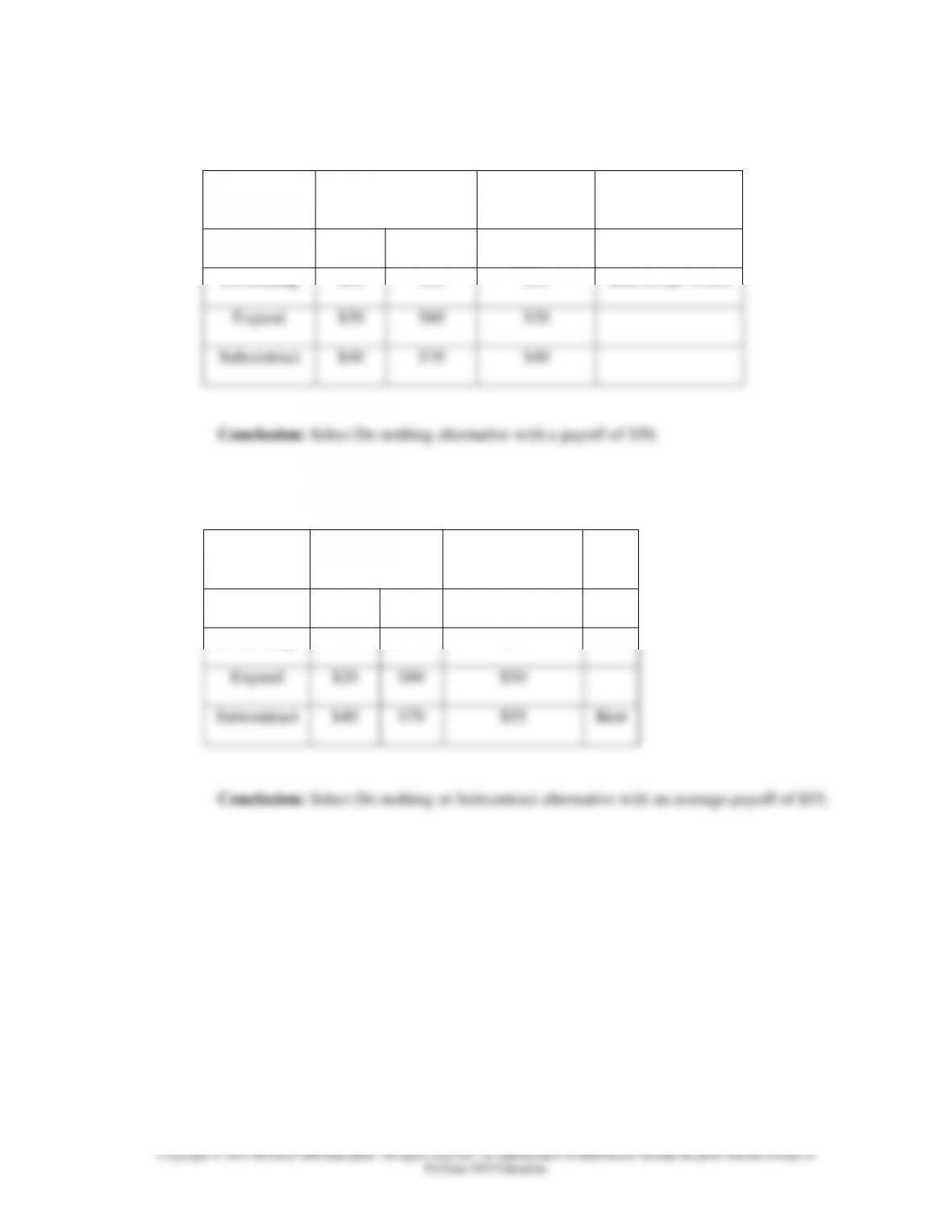
b. Maximin: Determine the worst possible payoff for each alternative and choose the
alternative that has the “best worst.”
Next Year’s
Demand
Alternative
Low
High
Worst Payoff
Do nothing
$50
$60
$50
Best of the Worst
Expand
$20
$80
$20
Subcontract
$40
$70
$40
Conclusion: Select Do nothing alternative with a payoff of $50.
c. Laplace: Determine the average payoff for each alternative and choose the alternative with
the best average.
$20
Subcontract
$40
$70
$55
Best
Next Year’s
Demand
Alternative
Low
High
Average Payoff
Do nothing
$50
$60
$55
Best
Chapter 05S – Decision Theory
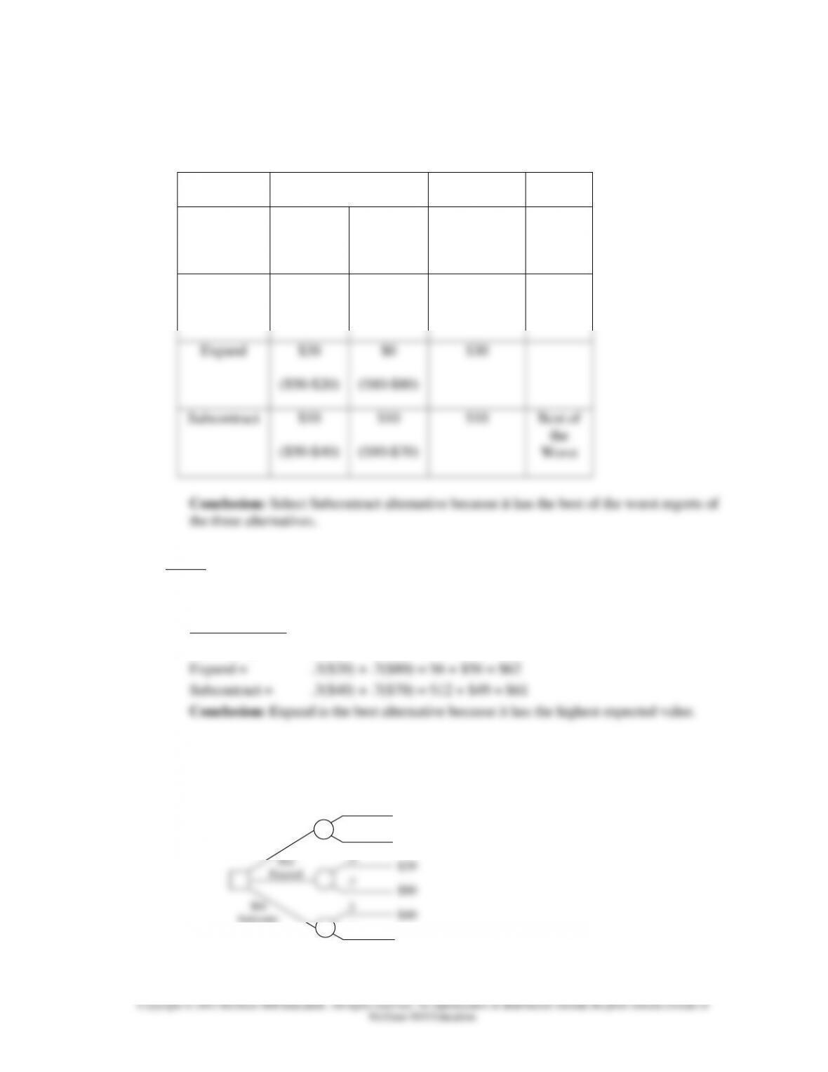
d. Minimax Regret: Prepare a table of regrets (opportunity losses)—for each column,
subtract every payoff from the best payoff in that column. Identify the worst regret for
each alternative. Select the alternative with the “best worst.”
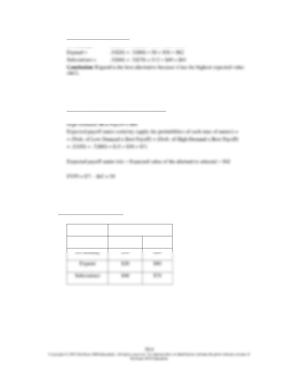
2. Given: P(Low Demand) = .3 and P(High Demand) = .7.
a. Determine the best expected profit of the alternatives from Problem 1
Expected Profit:
Do nothing = .3($50) + .7($60) = $15 + $42 = $57
b. Decision Tree Analysis to Select an Alternative:
Regrets
Alternative
Low
High
Worst
Regret
Do nothing
$0
($50-$50)
$20
($80-$60)
$20
.3
.7
.3
.7
$50
$60
$40
$70
$57
Do Nothing
Subcontr.
Chapter 05S – Decision Theory
Expected Value Calculations:
Do nothing = .3($50) + .7($60) = $15 + $42 = $57
c. Expected Value of Perfect Information:
Expected value of perfect information (EVPI) = Expected payoff under certainty –
Expected payoff under risk
Find the best payoff under each state of nature:
Low Demand: Best Payoff = $50
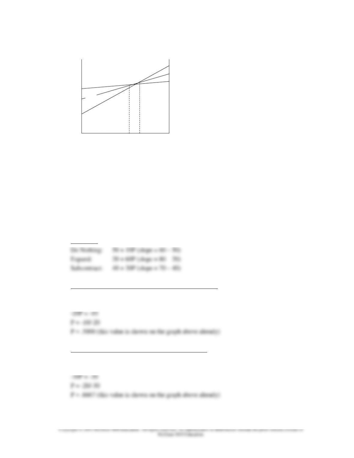
3. Plot each alternative relative to P(High Demand). Plot the payoff value for Low Demand on
the left side of the graph and the payoff value for High Demand on the right side of the graph.
Payoff values from Problem 1:
Next Year’s Demand
Alternative
Low
High
Do nothing
$50
$60
Expand
$20
$80
Subcontract
$40
$70
Chapter 05S – Decision Theory
5S-7
P(High)
The graph above shows the range of values of P(High) over which each alternative is optimal.
For low values of P(High), Do Nothing is best because it has the highest expected value.
For intermediate values of P(High), Subcontract is best.
For higher values of P(High), Expand is best.
To find the exact values of the ranges, we must determine where the upper parts of the lines
intersect. For each line, b is the slope of the line and x = P(High). The slope of each line =
Right-hand value – Left-hand value.
Equations:
Find the intersection between Do Nothing & Subcontract:
50 + 10P = 40 + 30P
10P – 30P = 40 – 50
Find the intersection between Subcontract & Expand:
40 + 30P = 20 + 60P
30P – 60P = 20 – 40
20
50
40
Do Nothing
Expand
0 .50 .6667 1.0
80
70
60
Low
Payoff
High
Payoff
Subcontract
Chapter 05S – Decision Theory
5S-8
Optimal ranges:
Do nothing: P(High) = 0 to < .5000
Subcontract: P(High) > .5000 to < .6667
Expand: P(High) > .6667 to 1.00
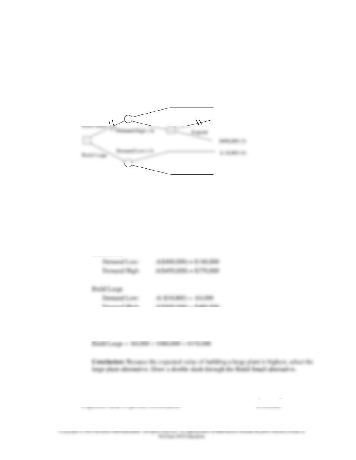
4. a. 1) Draw the tree diagram:
2) Analyze decisions from right to left (i.e., work backwards from the end of the tree
towards the root). For instance, begin with decision 2 and choose expansion because it
has a higher present value ($450,000 vs. $50,000). Draw a double slash through the
Maintain alternative.
3) Determine the product of the chance probabilities and their respective payoffs for the
remaining branches.
Build Small
Demand High: .6($800,000) = $480,000
4) Determine the expected value of each initial alternative.
Build Small = $160,000 + $270,000 = $430,000
b. Expected payoff under certainty: .4(400,000) + .6(800,000) = $640,000
-Expected payoff under risk: -476,000
$400,000 (1)
$50,000 (2)
$450,000 (3)
$-10,000 (4)
$800,000 (5)
Demand Low (.4)
Demand Low (.4)
Demand High (.6)
Demand High (.6)
Maintain
Expand
Build Small
Build Large
1
2
Chapter 05S – Decision Theory
5S-9
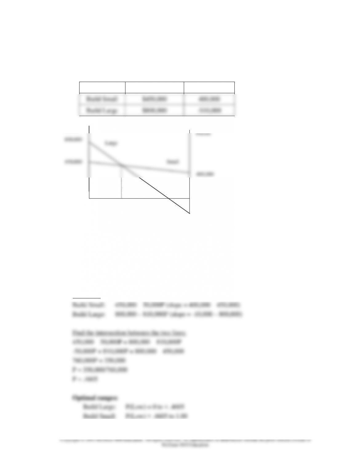
c. Determine the range over which each alternative would be best in terms of the value of
P(Low).
Plot each alternative relative to P(Low). Plot the payoff value for High Demand on the left
side of the graph and the payoff value for Low Demand on the right side of the graph.
Build Large
800,000
The graph above shows the range of values of P(Low) over which each alternative is optimal.
For low values of P(Low), Build Large is best because it has the highest expected value. For
high values of P(Low), Build Small is best because it has the highest expected value.
To find the exact values of the ranges, we must determine where the upper parts of the lines
intersect. For each line, b is the slope of the line and x = P(Low). The slope of each line =
Right-hand value – Left-hand value.
Equations:
Alternative
High Demand
Low Demand
-10,000
High
Payoff
Low
Payoff
P(Low)
0
1.0
Chapter 05S – Decision Theory
5S–10
5. Analyze the decisions from right to left:
1) Determine which alternative would be selected for each possible second decision.
Subcontract with Medium demand: Select either alternative. Payoff = $1.3.
Subcontract with Large demand: Select Build. Payoff = $1.8. Place a double slash through
Do nothing and Expand.
Build with Medium Demand: Select Other use #1. Payoff = $1.1. Place a double slash
through Do nothing and Other use #2.
2) Determine the product of the chance probabilities and their respective payoffs for the
remaining branches.
Subcontract
Small demand: .4($1.0) = $0.40
Expand
Small demand: .4($1.5) = $0.60
Medium demand: .5($1.6) = $0.80
Large demand: .1($1.7) = $0.17
Build
3) Determine the expected value of each initial alternative.