Chapter 03 – Forecasting
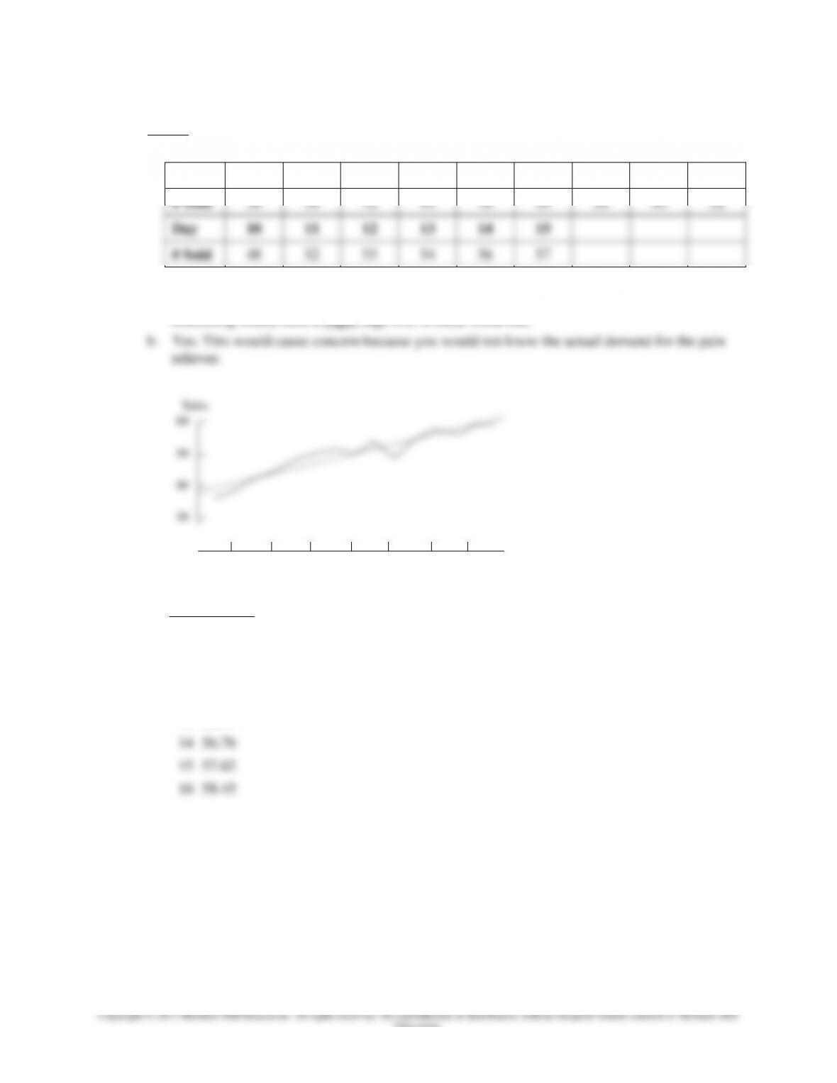
17. Given:
Day
1
2
3
4
5
6
7
8
9
# Sold
36
38
42
44
48
49
50
49
52
Day
10
11
12
13
14
15
# Sold
48
52
55
54
56
57
a. The trend may be non-linear (although most students will view it as linear). Trend-adjusted
smoothing would have a slight edge over a linear trend line.
Chapter 03 – Forecasting
3–22
Education.
Period
Actual
St-1 + Tt-1 = TAFt
TAFt + .3(At – TAFt) = St
Tt–1 + .3 (TAFt – TAFt–1 – Tt–1) = Tt
ei
ei2
8
49
50.00 (given)
50.00 + .3(49 – 50.00) = 49.70
2.00 (given)
-1.00
1.00
9
52
49.70 + 2.00 = 51.70
51.70 + .3(52 – 51.70) = 51.79
2.00 + .3(51.70 – 50.00 – 2.00) = 1.91
0.30
0.09
10
48
51.79 + 1.91 = 53.70
53.70 + .3(48 – 53.70) = 51.99
1.91 + .3(53.70 – 51.70 – 1.91) = 1.94
-5.70
32.49
11
52
51.99 + 1.94 = 53.93
53.93 + .3(52 – 53.93) = 53.35
1.94 + .3(53.93 – 53.70 – 1.94) = 1.43
-1.93
3.72
12
55
53.35 + 1.43 = 54.78
54.78 + .3(55 – 54.78) = 54.85
1.43 + .3(54.78 – 53.93 – 1.43) = 1.26
0.22
0.05
13
54
54.85 + 1.26 = 56.11
56.11 + .3(54 – 56.11) = 55.48
1.26 + .3(56.11 – 54.78 – 1.26) = 1.28
-2.11
4.45
14
56
55.48 + 1.28 = 56.76
56.76 + .3(56 – 56.76) = 56.53
1.28 + .3(56.76 – 56.11 – 1.28) = 1.09
-0.76
0.58
15
57
56.53 + 1.09 = 57.62
57.62 + .3(57 – 57.62) = 57.43
1.09 + .3(57.62 – 56.76 – 1.09) = 1.02
-0.62
0.38
16
57.43 + 1.02 = 58.45
Sum
42.76
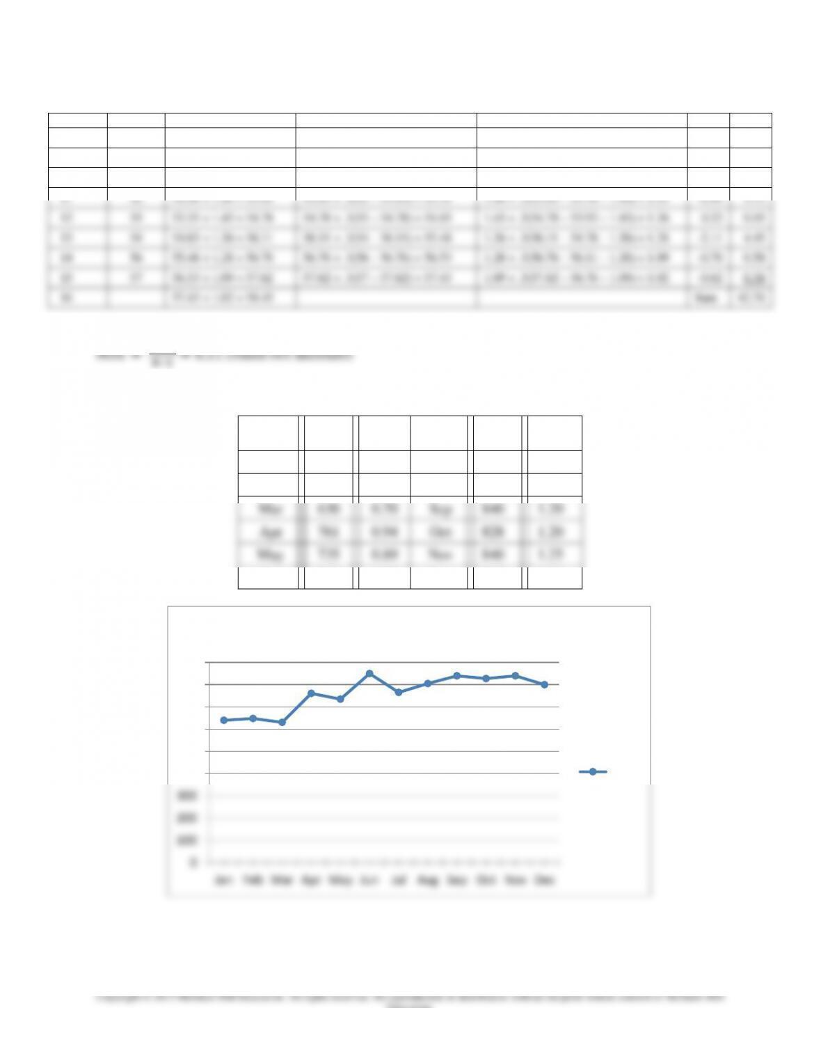
18. a. As shown in the plot of Unit Sales, there appears to be a trend in Unit Sales.
Month
Units
Sold
Index
Month
Units
Sold
Index
Jan
640
0.80
Jul
765
0.90
Feb
648
0.80
Aug
805
1.15
Mar
630
0.70
Sep
840
1.20
Apr
761
0.94
Oct
828
1.20
May
735
0.89
Nov
840
1.25
Jun
850
1.00
Dec
800
1.25
0
100
200
300
400
500
600
700
800
900
Jan Feb Mar Apr May Jun Jul Aug Sep Oct Nov Dec
Unit Sales
Units
Chapter 03 – Forecasting
3–23
Education.
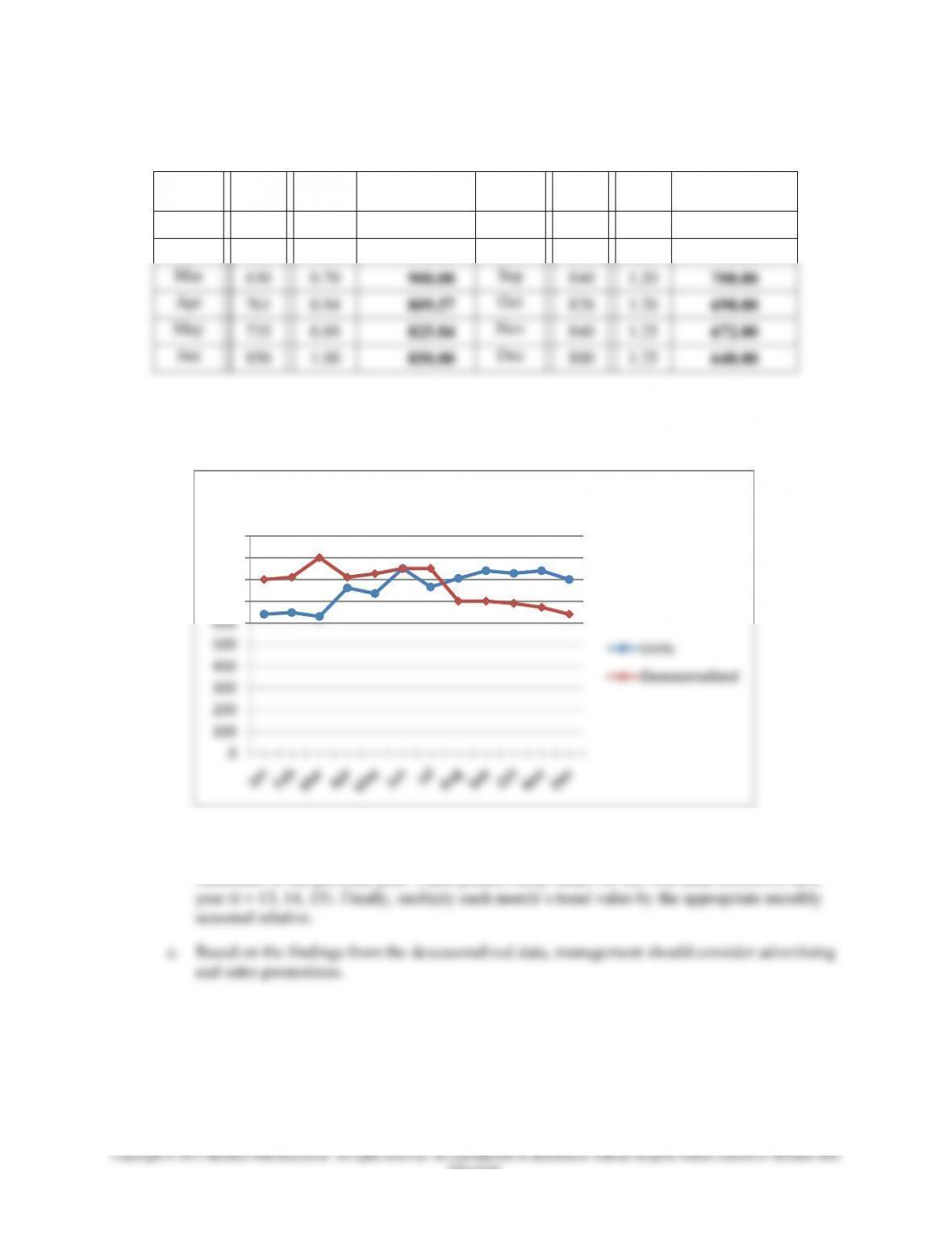
b. Deseasonalize car sales: Units Sold / Index (round to two decimals)
Month
Units
Sold
Index
Deseasonalized
Month
Units
Sold
Index
Deseasonalized
Jan
640
0.80
800.00
Jul
765
0.90
850.00
Feb
648
0.80
810.00
Aug
805
1.15
700.00
Mar
630
0.70
900.00
Sep
840
1.20
700.00
Apr
761
0.94
809.57
Oct
828
1.20
690.00
May
735
0.89
825.84
Nov
840
1.25
672.00
Jun
850
1.00
850.00
Dec
800
1.25
640.00
c. Plotting the deseasonalized data on the same graph as the Units Sold data leads us to a
different conclusion than the conclusion in part a. There appears to be a downward trend in
sales.
d. Part c indicated a downward trend in sales. We could forecast sales of the first three months
of the next year by fitting a monthly trend line to the deseasonalized values using t = 0 in
December of the previous year. Then, predict trend values for the first three months of next
0
100
200
300
400
500
600
700
800
900
1000
Unit Sales & Deseasonalized Data
Units
Deseasonalized

3–24
Education.
19. Deseasonalize the values, where:
Deseasonalized sales = (Actual sales) / (Seasonal relative) (round to two decimals):
Deseasonalized sales for quarter 1: 88/1.10 = 80.00
quarter of next year: (140.00 + 20) * 1.10 = 176.00.
20.
t
Units
sold
Naïve
e
| e |
e2
Trend F
e
| e |
e2
11
147
146
1
1
1
12
148
147
1
1
1
148
0
0
0
13
151
148
3
3
9
150
1
1
1
14
145
151
–6
6
36
152
–7
7
49
15
155
145
10
10
100
154
1
1
1
16
152
155
–3
3
9
156
–4
4
16
17
155
152
3
3
9
158
–3
3
9
18
157
155
2
2
4
160
–3
3
9
19
160
157
3
3
9
162
–2
2
4
20
165
160
5
5
25
164
1
1
1
Sum
18
36
202
–16
23
91
Round MAD & MSE to two decimals:
25.25
19
202
:
00.4
9
36
:
MSE
MAD
11.10
110
91
:
30.2
10
23
:
MSE
MAD

Chapter 03 – Forecasting
3–25
Education.
21.
Period
Demand
F1
e
e
e2
(e/Demand)
x 100 (%)
F2
e
e
e2
(e/Demand)
x 100 (%)
1
68
66
2
2
4
2.94%
66
2
2
4
2.94%
2
75
68
7
7
49
9.33%
68
7
7
49
9.33%
3
70
72
–2
2
4
2.86%
70
0
0
0
0.00%
4
74
71
3
3
9
4.05%
72
2
2
4
2.70%
5
69
72
–3
3
9
4.35%
74
–5
5
25
7.25%
6
72
70
+2
2
4
2.78%
76
–4
4
16
5.56%
7
80
71
9
9
81
11.25%
78
2
2
4
2.50%
8
78
74
4
4
16
5.13%
80
–2
2
4
2.56%
Sum
32
176
42.69%
24
106
32.84%
a. MAD F1: 32/8 = 4.00 (round to two decimals)
MAD F2: 24/8 = 3.00 (F2 appears to be more accurate)
MAD would be more natural.
d. MAPE calculations (round to two decimals):
MAPE (F1): 42.69%/8 = 5.34%
MAPE (F2): 32.84%/8 = 4.11%
Because 4.11% < 5.34%, F2 appears to be more accurate.

Chapter 03 – Forecasting
3–26
Education.
22. a. Compute MSE & MAD for each forecast method (round to two decimals). Round % to two
decimals.
Period
Demand
F1
e
e
e2
(e/Demand)
x 100 (%)
F2
e
e
e2
(e/Demand)
x 100 (%)
1
770
771
-1
1
1
0.13%
769
1
1
1
0.13%
2
789
785
4
4
16
0.51%
787
2
2
4
0.25%
3
794
790
4
4
16
0.50%
792
2
2
4
0.25%
4
780
784
-4
4
16
0.51%
798
–18
18
324
2.31%
5
768
770
-2
2
4
0.26%
774
-6
6
36
0.78%
6
772
768
4
4
16
0.52%
770
2
2
4
0.26%
7
760
761
-1
1
1
0.13%
759
1
1
1
0.13%
8
775
771
4
4
16
0.52%
775
0
0
0
0.00%
9
786
784
2
2
4
0.25%
788
-2
2
4
0.25%
10
790
788
2
2
4
0.25%
788
2
2
4
0.25%
Sum
12
28
94
3.58%
–16
36
382
4.61%
MAD F1: 28/10 = 2.80
MAD F2: 36/10 = 3.60
b. Compute MAPE for each forecast method (round to two decimals).

Chapter 03 – Forecasting
3–27
Education.
c. Naïve Method Forecast
Month
Sales
Naïve
Forecast
e
| e |
e2
1
770
2
789
770
19
19
361
3
794
789
5
5
25
4
780
794
–14
14
196
5
768
780
–12
12
144
6
772
768
4
4
16
7
760
772
–12
12
144
8
775
760
15
15
225
9
786
775
11
11
121
10
790
786
4
4
16
11
790
At end of
Week 10
20
96
1,248
Round MSE, MAD, TS, & control limits to two decimals:
It appears that the naïve forecast is in control because its tracking signal at the end of Week
10 is within the limits. However, the MAD and MSE values for the naïve method are much
higher than the MAD and MSE values for the other two forecasting methods (refer to the
table below). Therefore, the naïve forecasting method does not appear to be performing as
well as the other two forecasting methods.
Method
MAD
MSE
F1
2.80
10.44
F2
3.60
42.44
Naïve
10.67
156.00
Chapter 03 – Forecasting
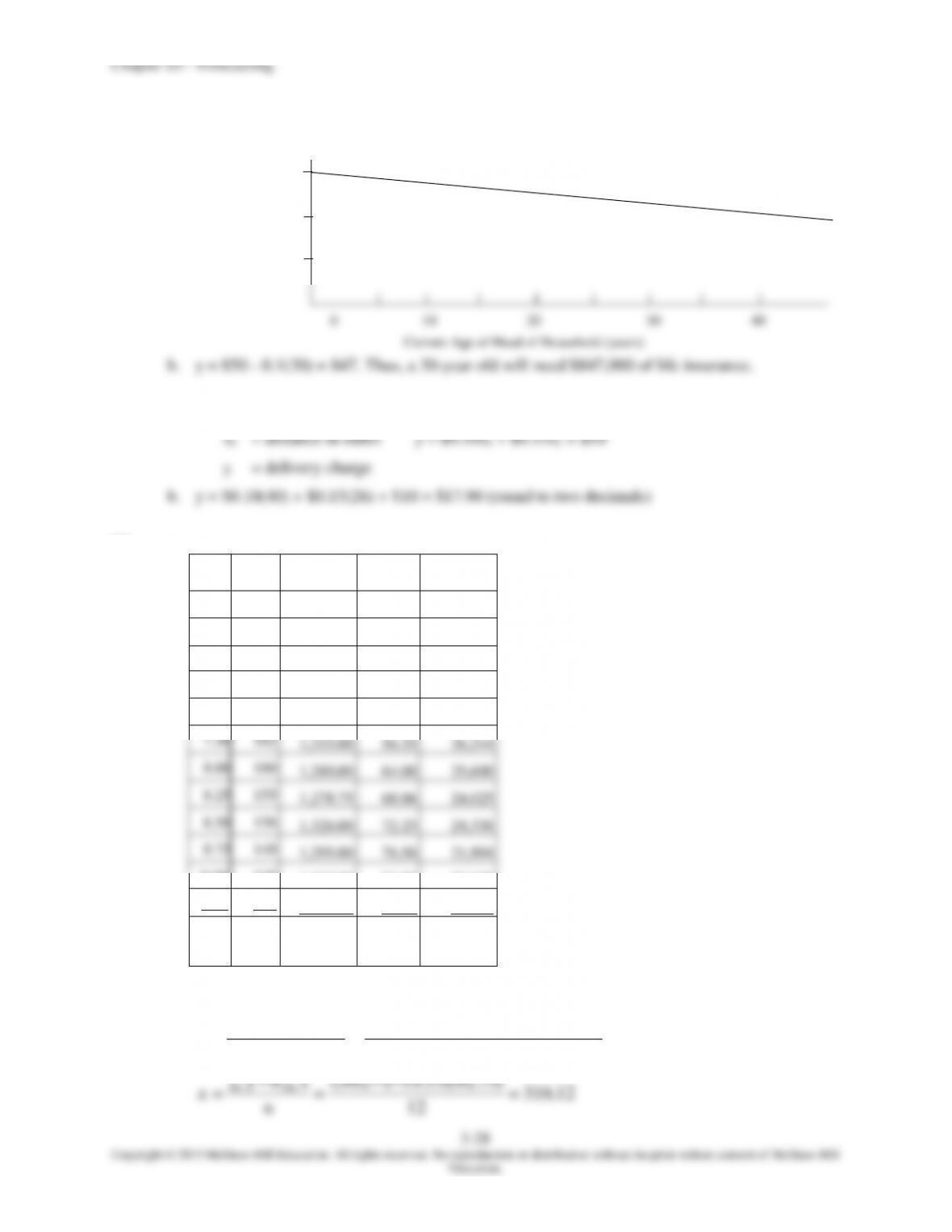
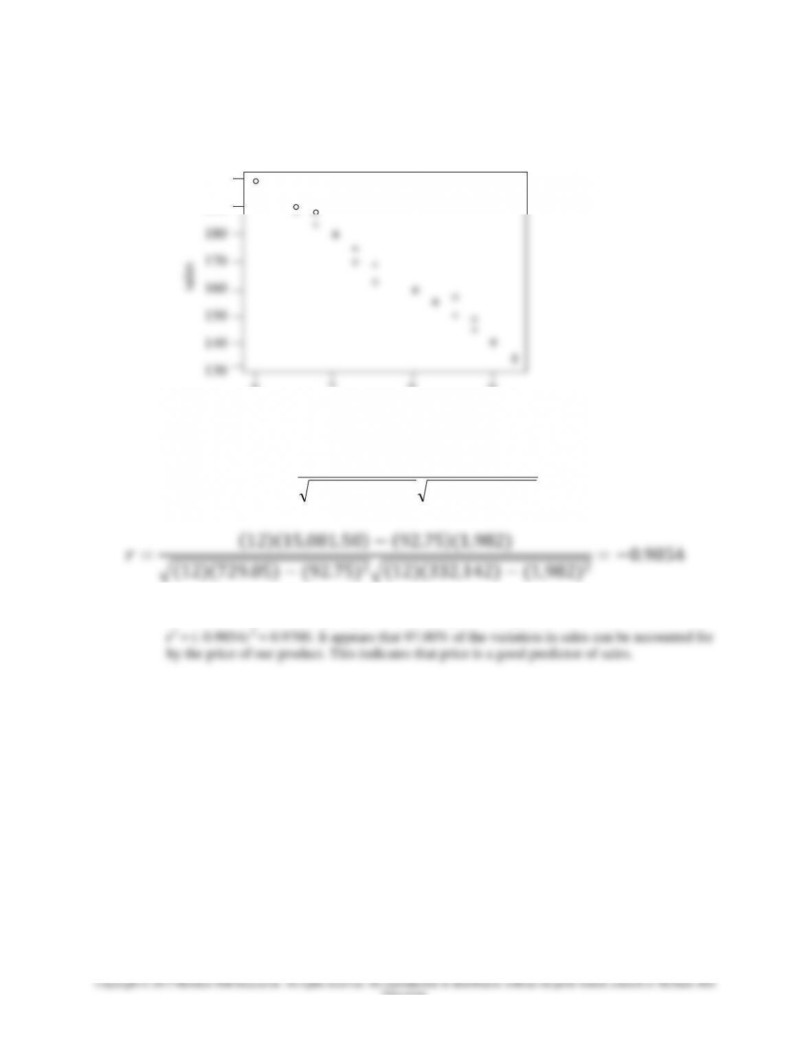
Y = 316.12 – 19.53X
Actual data are represented by circles.
Predicted values are represented by pluses.
+
+
+
+
+
+
+
Round r to four decimals:
2222 )()()()(
))(()(
yynxxn
yxxyn
r
b. r = –0.9854 implies a strong, negative relationship between price and demand.
6 7 8 9
price
200
190
130
+
Chapter 03 – Forecasting
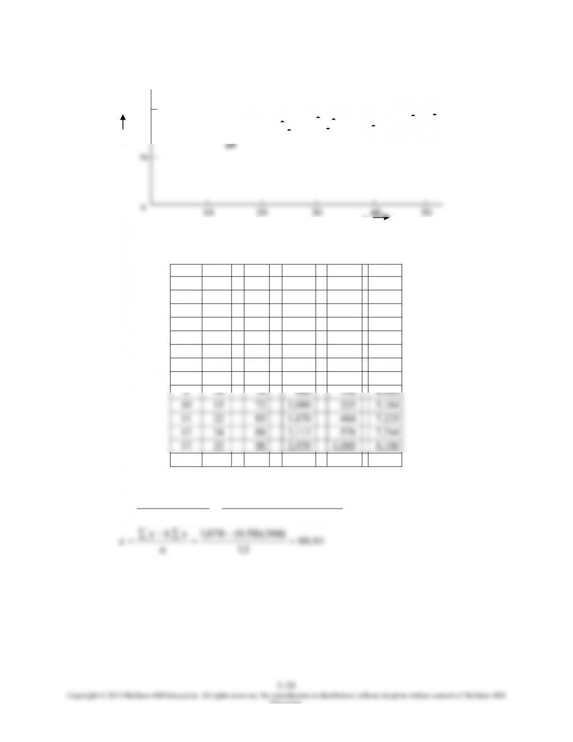
26. a.
b.
t
x
y
x * y
x2
y2
1
15
74
1,110
225
5,476
2
25
80
2,000
625
6,400
3
40
84
3,360
1,600
7,056
4
32
81
2,592
1,024
6,561
5
51
96
4,896
2,601
9,216
6
47
95
4,465
2,209
9,025
7
30
83
2,490
900
6,889
8
18
78
1,404
324
6,084
9
14
70
980
196
4,900
10
15
72
1,080
225
5,184
11
22
85
1,870
484
7,225
12
24
88
2,112
576
7,744
13
33
90
2,970
1,089
8,100
366
1,076
31,329
12,078
89,860
Round b & a to two decimals:
58.0
)366()078,12)(13(
)076,1)(366()329,31)(13(
)( 222
xxn
yxxyn
b
10 20 30 40 50
0
y
x
100