
Chapter 03 – Forecasting
3-1
CHAPTER 03
FORECASTING
Forecasting is placed early in the text mainly because it is a point of departure. Some instructors like to
emphasize the operations part of operations management and de-emphasize the design part. Other
instructors prefer to blend the two. However, forecasting is an important input for both, and for that
reason, it is presented as early as possible.
Teaching Notes
This is a long chapter, so you may want to be selective about the topics covered to shorten the time
devoted to it. I tend to devote more time to the time series methods than I do to regression analysis, for
several reasons. One is that students often are exposed to regression in their stat course(s). Another is that
time series models are used more than associative models are. Other optional materials that can be
mentioned briefly, but not explored in detail, include trend-adjusted exponential smoothing (mentioned so
that students will realize that exponential smoothing does not work well if there is trend present) and
computation of seasonal relatives (you may want to explain how relatives are used without getting into
how they are derived).
I try to emphasize an intuitive approach to forecasting, with frequent reference to the importance of
plotting the data to assist the decision-maker in determining which forecasting technique may be more
appropriate to use.
In operations management, we forecast a wide range of future events, which could significantly affect the
long-term success of the firm. Most often, the basic need for forecasting arises in estimating customer
demand for a firm’s products and services. However, we may need aggregate estimates of demand as well
as estimates for individual products. In most cases, a firm will need a long-term estimate of overall
demand as well as a shorter-run estimate of demand for each individual product or service. Short-term
demand estimates for individual products are necessary to determine daily or weekly management of the
demand, while an active response would be to advertise in an effort to offset the predicted decrease in
demand.
Reading: Gazing at the Crystal Ball
1. Demand forecasting (DF) is part science and part art (intuition) for estimating what future
demand for a product or service will be. The science part uses information technology to generate
2. A company executive might make bold predictions about future demand to Wall Street analysts to
maintain the company’s stock price.

Chapter 03 – Forecasting
3-2
Education.
3. An executive’s comments to Wall Street analysts may result in the company changing its demand
forecast to reflect the comments made by the executive. The result often is excessive inventory
build-up starting at the distribution channels to the upstream suppliers.
Answers to Discussion and Review Questions
1. It depends on the situation at hand. In certain situations, one approach will be superior to the
other.
2. Poor forecasting leads to poor planning. This could result in offering products and services that
3. a. Consumer surveys may be invalid if they are not carefully constructed, administered, and
interpreted. Moreover, respondents may be ill informed or otherwise formulate answers that
4. Forecasts generally are wrong due to the use of an incorrect model to forecast, random variation,
or unforeseen events.
5. Control limits reveal the bounds of random errors; they enable managers to judge if a forecasting
technique is performing as well as it might (and hence, when a technique should be reevaluated).
6. The relative costs of reevaluating a forecast when nothing is wrong versus not reevaluating it
7. MAD focuses on average error while MSE focuses on squared errors. (MSE gives considerably
more weight to large forecast errors.)
8. Exponential smoothing: requires less data storage, gives more weight to recent data, and is easier
to change to make it more responsive to changes in demand.
9. The fewer the periods in a moving average, the greater the responsiveness.
10. The choice of alpha in exponential smoothing depends on how responsive a forecast the manager
Chapter 03 – Forecasting
11. Of course, the accuracy of your five-day weather forecast will depend on a number of variables
such as time of year, where you live, etc. However, there is one trend that will establish itself and
that is as time passes from the first day to the fifth day, the accuracy of the forecast will decline.
12. For example, if each average is based on 12 months, as each new data point is added to the
moving average, its counterpart is removed from the other end of the series.
13. Sales indicate how much customers bought, while demand indicates how much they wanted. The
14. A reactive approach takes the forecast as a “given” while a proactive approach takes an
unacceptable forecast and attempts to alter demand. An example of the reactive approach is a
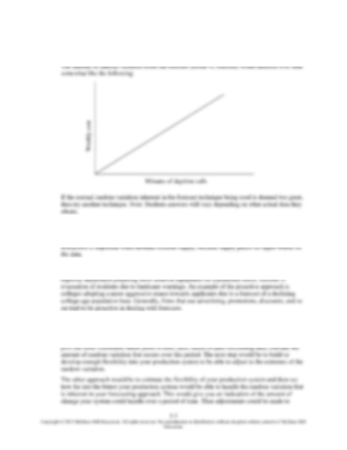
15. There is always going to be a certain amount of random variation about the forecast. The amount
of this random variation about the forecast (actual vs. forecast) will increase as the forecasting
horizon is extended. In other words, forecasting accuracy tends to decline over time.
Consequently, one of two approaches might be employed to handle the problem. One would be to
3-4
Copyright © 2015 McGraw-Hill Education. All rights reserved. No reproduction or distribution without the prior written consent of McGraw-Hill
Education.
16. Forecasting in the context of supply chain involves connection and communication between the
supply chain databases. For example, assume that Company X is a durable goods manufacturer.
Based on the market and historical sales information, Company X determines short and
17. It depends on the situation. Sometimes one approach is better, sometimes the other is better, and
sometimes both are used. Considerations include the importance of the forecasts, how quickly the
18. In forecasting initial sales for the new version of its software, the software producer should
consider:
a. The historical demand information for the old version.
19. a. Demand for Mother’s Day greeting cards: Naïve using last year’s demand. Alternatively,
because greeting cards have seasonal demand, we could use a seasonal model where the
season begins a few weeks before Mother’s Day and ends just after Mother’s Day.
Chapter 03 – Forecasting
Taking Stock
1. If the forecast system is too responsive and it becomes too sensitive to the changes in actual
2. Forecasting needs to be a collaborative effort involving marketing, operations, and technical
3. The technology has had tremendous impact on forecasting mainly because of the advancement of
the computer technology. Computer technology plays a very important role in preparing forecasts
based on quantitative data. Computer technology allows companies to generate forecasts quickly
due to the computer system’s enhanced ability to update information on prices, demand, and other
variables. In addition, the ability to integrate databases along the supply chain has proved to be an
invaluable asset to companies because this feature increases the communication between
suppliers and their customers, resulting in better management of inventories and purchase orders.
Critical Thinking Exercises
1. The conditions that would have to exist for driving a car that are analogous to the assumptions
made when using exponential smoothing are that the immediate future will be like the recent past.
This would suggest:
a. No sharp curves or turns on the road
d. Constant road conditions
2. Instantaneous re-supply and/or completely flexible capacity.
3. Potential investors would expect information on the current and future size of the market, the
expected initial market share and growth rate for 5-10 years, profit/loss projections for the
4. How to handle a poor forecast (i.e., one that is substantially above or below actual demand)
would depend on what the items is, and on a number of factors. For example, a low forecast
would lead to a stockout. How critical that is would relate to how important that a stockout is to
5. Although understandable, Omar’s approach is not ethical. He should turn in the forecast based on
the information he has and tell his superiors that he thinks he can get those numbers up. The only
pro to Omar’s optimistic forecast might be preventing Oscar from being laid off over the near-
3-6
Education.
6. Student answers will vary. Some possibilities follow:
a. If an executive lied and was overly optimistic about demand forecasts, this would violate the
Utilitarian Principle and the Virtue Principle.
b. If an executive forced a subordinate to adjust a forecast based on arbitrary reasons, this would
violate the Rights Principle.
Chapter 03 – Forecasting
3-7
Education.
Solutions
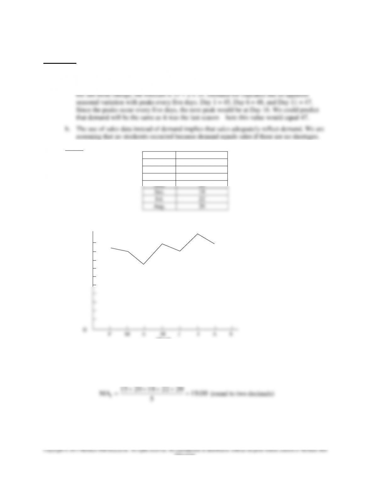
1. a. Plotting each data set reveals that blueberry muffin orders are stable, varying around an
average. Therefore, the naïve forecast is the last value, 33. The demand for cinnamon buns
has a trend. The last change was from 31 to 33 (33 – 31 = 2). Using the last value and adding
2. Given:
Month
Sales (000 units)
Feb.
19
Mar.
18
Apr.
15
May
20
Jun.
18
Jul.
22
Aug.
20
a.
b. 1) Using the naïve approach, the forecast for the next month (September) will equal 20.
2) A five-month moving average is shown below:
2022182015
Month
Sales
20
3-8
3) A weighted using average using 0.60 for August, 0.30 for July, and 0.10 for June is shown
below:
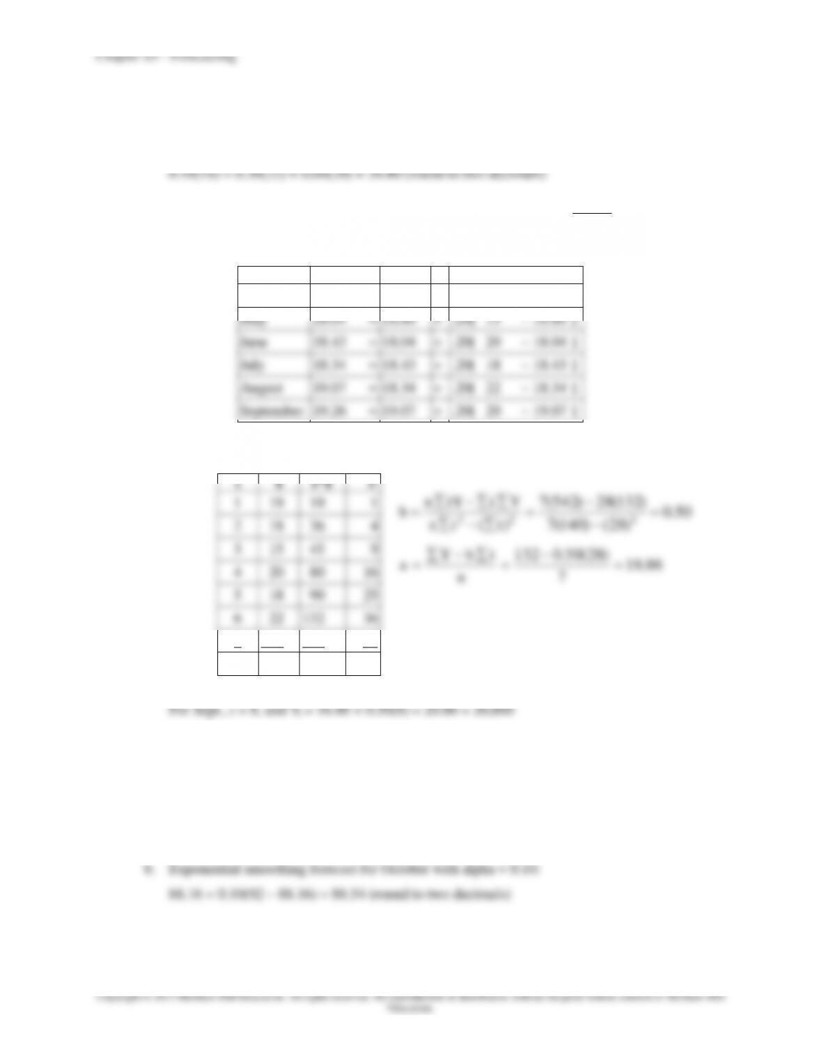
4) Exponential smoothing, with alpha = 0.20 and an initial forecast for March of 19 are shown
below (round to two decimals):
Month
Forecast =
F(old)
+
.20[Actual – F(old)]
April
18.80 =
19
+
.20[ 18 – 19 ]
May
18.04 =
18.80
+
.20[ 15 – 18.80 ]
June
18.43 =
18.04
+
.20[ 20 – 18.04 ]
July
18.34 =
18.43
+
.20[ 18 – 18.43 ]
August
19.07 =
18.34
+
.20[ 22 – 18.34 ]
September
19.26 =
19.07
+
.20[ 20 – 19.07 ]
5) A linear trend forecast is shown below (round b & a to two decimals):
t
Y
t*Y
t2
50.0
)28()140(7
)132(28)542(7
)( 222
ttn
YttYn
b
86.16
7
)28(50.0132
n
tbY
a
1
19
19
1
2
18
36
4
3
15
45
9
4
20
80
16
5
18
90
25
6
22
132
36
7
20
140
49
28
132
542
140
c. The linear trend approach seems to be the least appropriate because the data appear to vary
around an average of about 19 [18.86] and because the slope is close to zero (0.50).
d. Sales are reflective of demand (i.e., no stockouts or backorders occurred).
3. a. Exponential smoothing forecast for September with alpha = 0.10:
88 + 0.10(89.6 – 88) = 88.16 (round to two decimals)
Chapter 03 – Forecasting
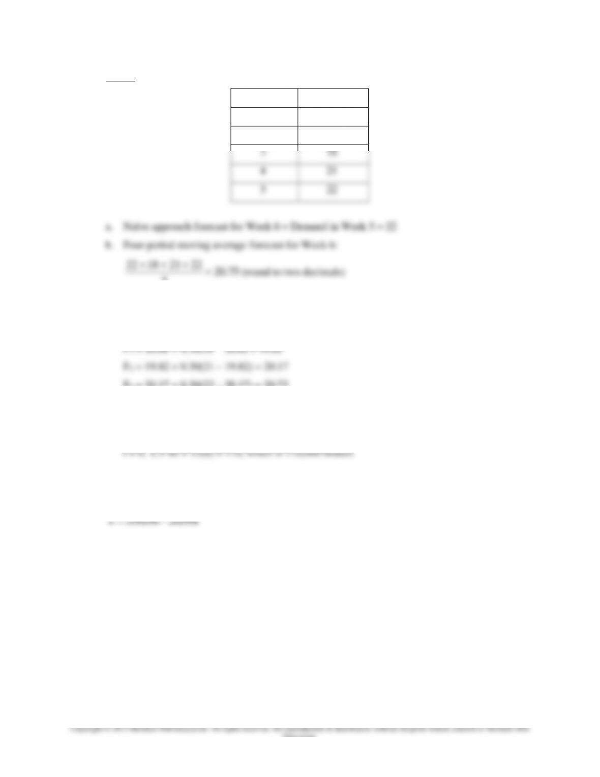
4. Given:
Week
Requests
1
20
2
22
3
18
4
21
5
22
3–10
Education.
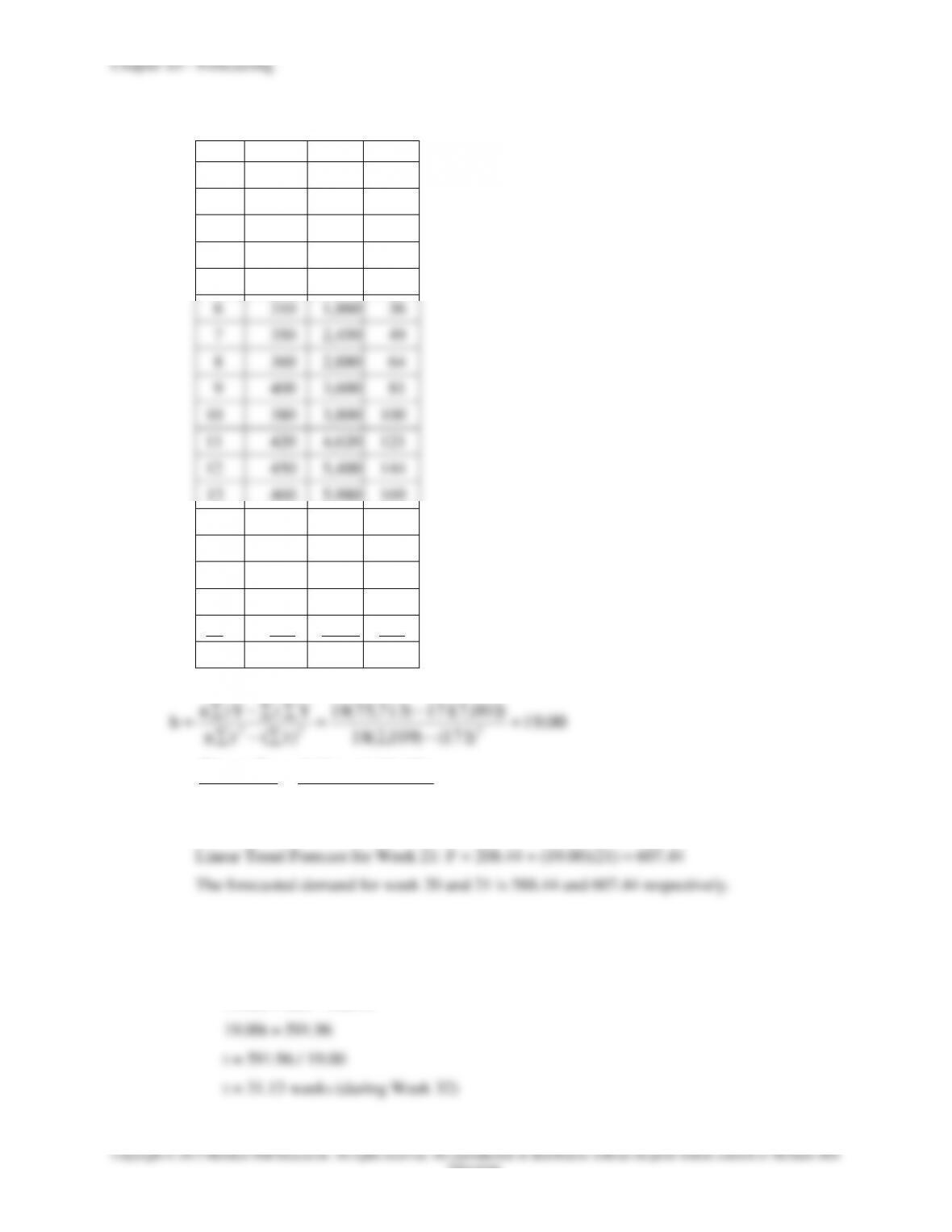
7.
a.
t
Y
t*Y
t2
1
220
220
1
2
245
490
4
3
280
840
9
4
275
1,100
16
5
300
1,500
25
6
310
1,860
36
7
350
2,450
49
8
360
2,880
64
9
400
3,600
81
10
380
3,800
100
11
420
4,620
121
12
450
5,400
144
13
460
5,980
169
14
475
6,650
196
15
500
7,500
225
16
510
8,160
256
17
525
8,925
289
18
541
9,738
324
171
7,001
75,713
2,109
00.19
)171()109,2(18
)001,7(171)713,75(18
)( 222
ttn
YttYn
b
44.208
18
)171(00.19001,7
n
tbY
a
b. Linear Trend Forecast for Week 20: F = 208.44 + (19.00)(20) = 588.44
c. Set the trend equation = 800 and solve for t:
208.44 + 19.00t = 800
19.00t = 800 – 208.44