Chapter 19 – Linear Programming
19–81
Table 2 Completed Initial Tableau.
C
4
5
0
0
Variables
in solution
x1
x2
s1
s2
Solution
quantity
0
s1
1
3
1
0
12
0
s2
4
3
0
1
24
Z
0
0
0
0
0
C – Z
4
5
0
0
Table 3
C
4
5
0
0
Variables
in solution
x1
x2
s1
s2
Solution
quantity
0
s1
1
3
1
0
12/3 = 4
0
s2
4
3
0
1
24/3 = 8
Z
0
0
0
0
0
C – Z
4
5
0
0
Largest
+ ratio
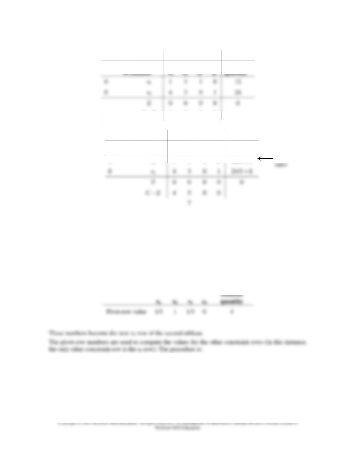
At this point we can begin to develop the second tableau. The row of the leaving variable will be
transformed into the new pivot row of the second tableau. This will serve as a foundation on which to
develop the other rows. To obtain this new pivot row, we simply divide each element in the s1 row by
the row pivot value (intersection of the entering column and leaving row), which is 3. The resulting
numbers are:
x1
x2
s1
s2
Solution
quantity
Pivot-row value
1/3
1
1/3
0
4
These numbers become the new x2 row of the second tableau.
The pivot-row numbers are used to compute the values for the other constraint rows (in this instance,
the only other constraint row is the s2 row). The procedure is:
1. Find the value that is at the intersection of the constraint row (i.e., the s2 row) and the entering
variable column. It is 3.
2. Multiply each value in the new pivot row by this value.
3. Subtract the resulting values, column by column, from the current row values.
Smallest +
ratio
Chapter 19 – Linear Programming
x1
x2
s1
s2
Quantity
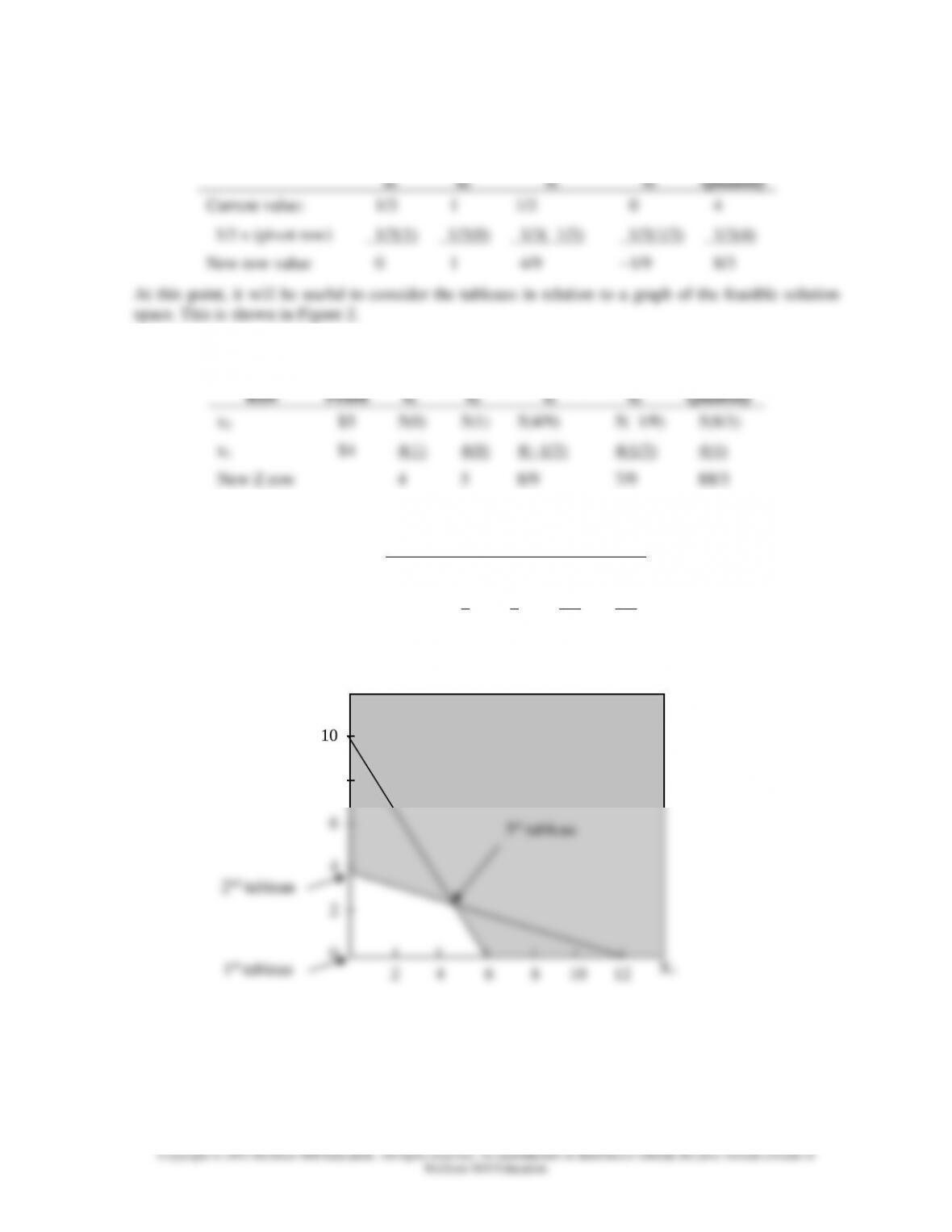
Current value:
4
3
0
1
24
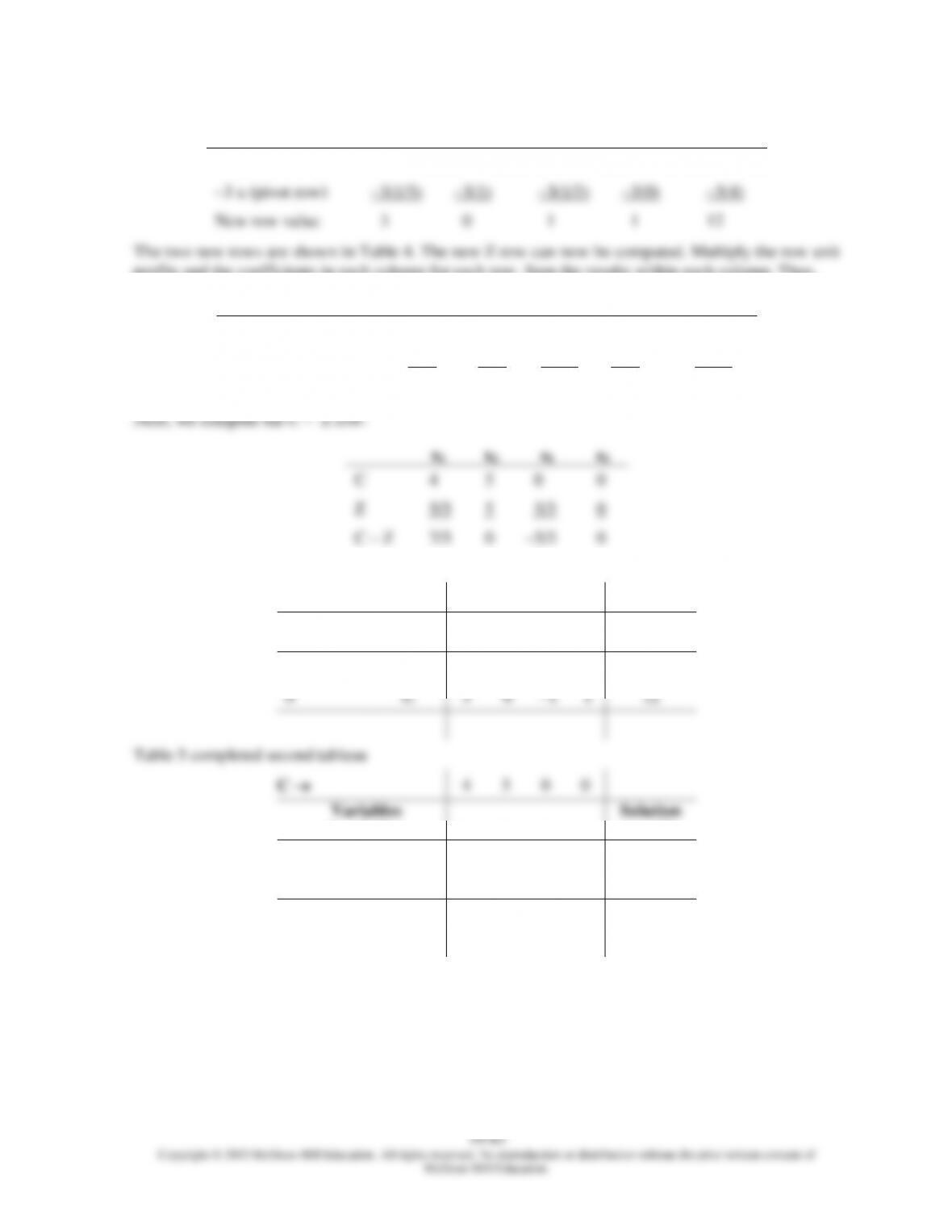
–3 x (pivot row)
–3(1/3)
–3(1)
–3(1/3)
–3(0)
–3(4)
New row value
3
0
–1
1
12
The two new rows are shown in Table 4. The new Z row can now be computed. Multiply the row unit
profits and the coefficients in each column for each row. Sum the results within each column. Thus,
Row
Profit
x1
x2
s1
s2
Quantity
x2
5
5(1/3)
5(1)
5(1/3)
5(0)
5(4)
s1
0
0(3)
0(0)
0(–1)
0(1)
0(12)
New Z row
5/3
5
5/3
0
20
x1
x2
s1
s2
C
4
5
0
0
Z
5/3
5
5/3
0
C – Z
7/3
0
–5/3
0
Table 4 partially completed second tableau
C
4
5
0
0
Variables
in solution
x1
x2
s1
s2
Solution
quantity
5
x2
1/3
1
1/3
0
4
0
s2
3
0
–1
1
12
Table 5 completed second tableau
C
4
5
0
0
Variables
in solution
x1
x2
s1
s2
Solution
quantity
5
x2
1/3
1
1/3
0
4
0
s2
3
0
–1
1
12
Z
5/3
5
5/3
0
20
C – Z
7/3
0
–5/3
0
Chapter 19 – Linear Programming
The completed second tableau is shown in Table 5. It tells us that at this point 4 units of variable x2 are
the most we can make (see column Solution quantity, row x2) and that the profit associated with x2 =
4, x1= 0 is $20 (see row Z, column Solution quantity).
The fact that there is a positive value in the C – Z row tells us that this is not the optimal solution.
Consequently, we must develop another tableau.
Developing the Third Tableau
The third tableau will be developed in the same manner as the previous one.
1. Determine the entering variable: Find the column with the largest positive value in the C – Z
row (7/3, in the x1 column).
Chapter 19 – Linear Programming
4. Compute values for the x2 row: Multiply each new pivot-row value by the x2 row pivot value
(i.e., 1/3) and subtract the product from corresponding current values. Thus,
x1
x2
s1
s2
Quantity
Current value:
1/3
1
1/3
0
4
–1/3 x (pivot row)
–1/3(1)
–1/3(0)
–1/3(–1/3)
–1/3(1/3)
–1/3(4)
New row value
0
1
4/9
–1/9
8/3
At this point, it will be useful to consider the tableaus in relation to a graph of the feasible solution
space. This is shown in Figure 2.
5. Compute new Z row values. Note that now variable x1 has been added to the solution mix; that
row’s unit profit is $4.
Row
Profit
x1
x2
s1
s2
Quantity
x2
$5
5(0)
5(1)
5(4/9)
5(–1/9)
5(8/3)
x1
$4
4(1)
4(0)
4(–1/3)
4(1/3)
4(4)
New Z row
4
5
8/9
7/9
88/3
6. Compute the C – Z row values:
x1
x2
s1
s2
C
4
5
0
0
Z
4
5
8/9
7/9
C – Z
0
0
–8/9
–7/9
Figure 2 Graphical Solution and Simplex Tableaus
X1
3rd tableau
10
8
6
4
2
0
2 4 6 8 10 12
X2
1st tableau
2nd tableau
Chapter 19 – Linear Programming
Table 7. Optimal Solution
C
4
5
0
0
Variables
in solution
x1
x2
s1
s2
Solution
quantity
5
x2
0
1
4/9
–1/9
8/3
4
x1
1
0
–1/3
1/3
4
Z
4
5
8/9
7/9
88/3
C – Z
0
0
–8/9
–7/9
The resulting values of the third tableau are shown in Table 7. Note that each of the C – Z
values is either 0 or negative, indicating that this is the final solution. The optimal values of x1
and x2 are indicated in the quantity column: x2 = 8/3, or 2 2/3, and x1 = 4. (The x2 quantity is
When an equality constraint is present, use of the simplex method requires addition of an artificial
variable. The purpose of such variables is merely to permit development of an initial solution. For
example, the equalities
(1) 7x1 + 4x2 = 65
(2) 5x1 + 3x2 = 40
where
M = A large number (e.g., 999)
Since the artificial variables are not desired in the final solution, selecting a large value of M (much
larger than the other objective coefficients) will insure their deletion during the solution process.
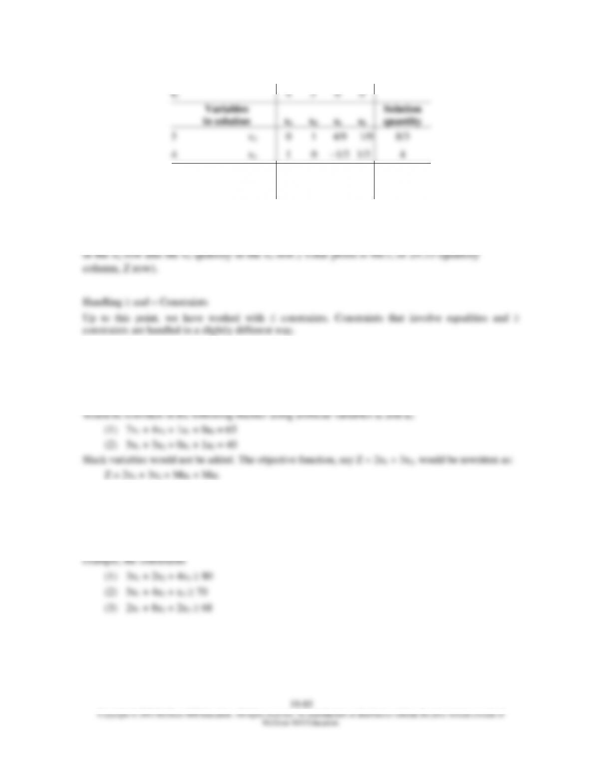
For constraints, surplus variables must be subtracted instead of added to each constraint. For
Chapter 19 – Linear Programming
19–86
would be rewritten as equalities:
(1) 3x1 + 2x2 + 4x3 – 1s1 – 0s2 – 0s3 80
(2) 5x1 + 4x2 + x3 – 0s1 – 1s2 – 0s3 70
(3) 2x1 + 8x2 + 2x3 – 0s1 – 0s2 – 1s3 + 0a1 + 0a2 + 1a3 68
If the objective function happened to be
5x1 + 2x2 + 7x3
it would become
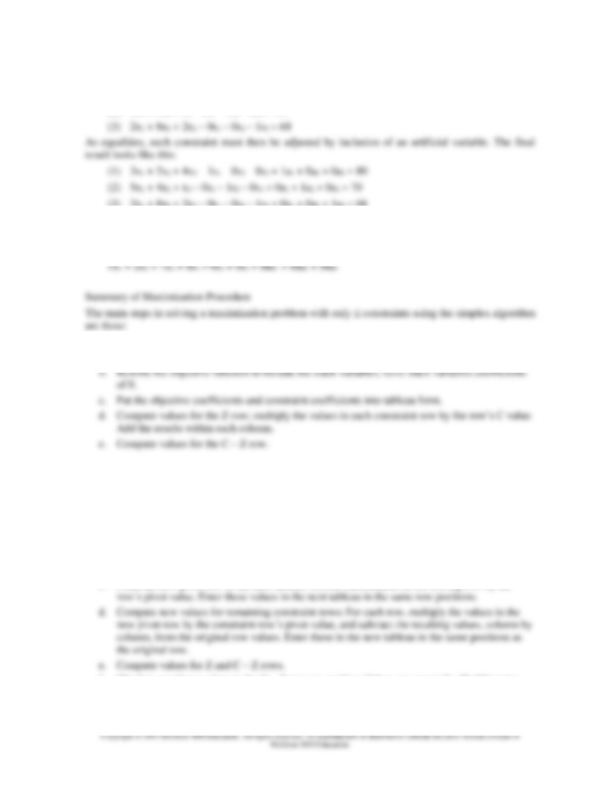
1. Set up the initial tableau.
a. Rewrite the constraints so that they become equalities; add a slack variable to each constraint.
2. Set up subsequent tableaus.
a. Determine the entering variable (the largest positive value in the C– Z row). If a tie exists,
choose one column arbitrarily.
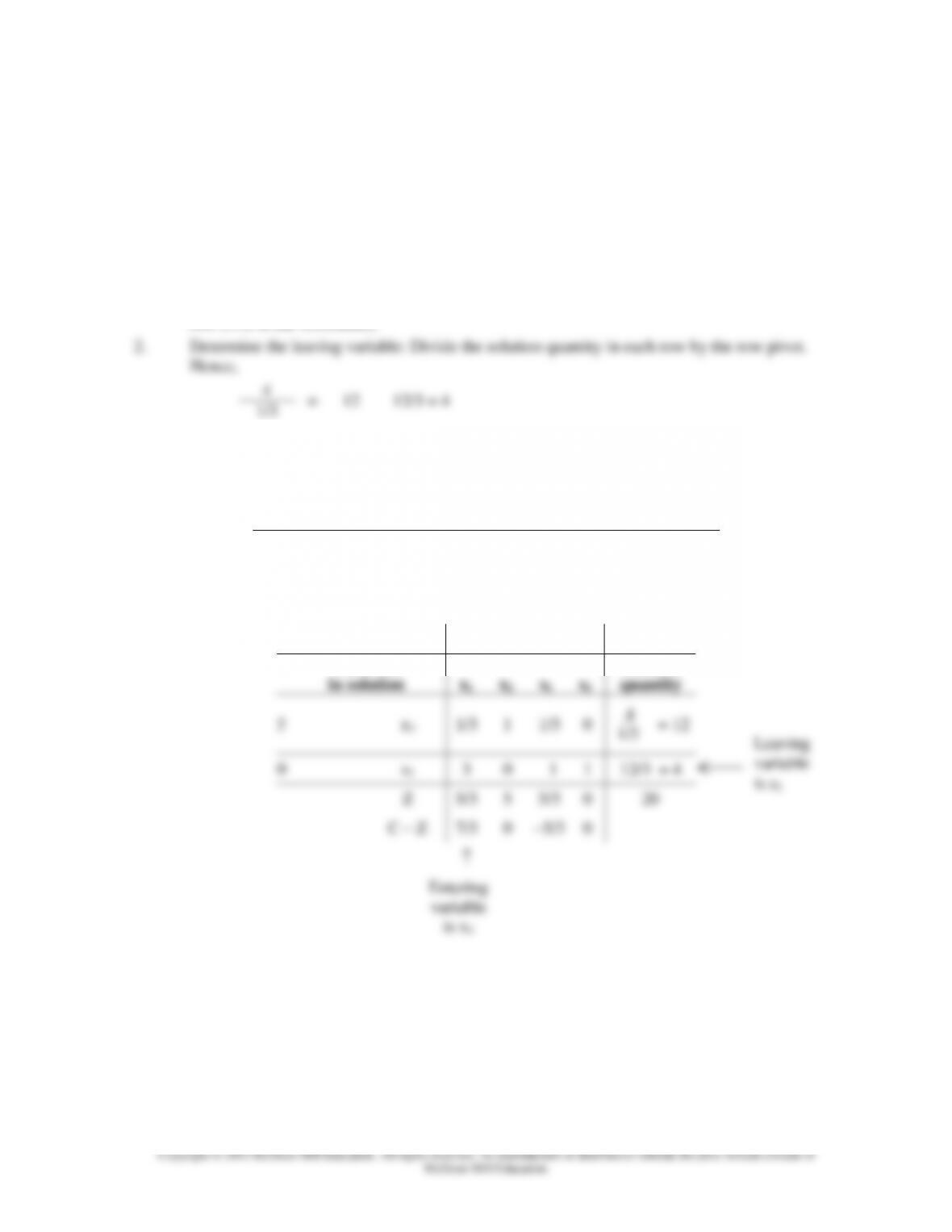
b. Determine the leaving variable: Divide each constraint row’s solution quantity by the row’s
pivot value; the smallest positive ratio indicates the leaving variable. If a tie occurs, divide the
values in each row by the row pivot value, beginning with slack columns and then other
columns, moving from left to right. The leaving variable is indicated by the lowest ratio in the
first column with unequal ratios.
c. Form the new pivot row of the next tableau: Divide each number in the leaving row by the
f. Check to see if any values in the C – Z row are positive; if they are, repeat 2a–2f. Otherwise,
the optimal solution has been obtained.
Chapter 19 – Linear Programming
Minimization Problems
The simplex method handles minimization problems in essentially the same way it handles
maximization problems. However, there are a few differences. One is the need to adjust for
solution more involved. A second major difference is the test for the optimum: A solution is optimal if
there are no negative values in the C – Z row.
Example
Solve the following problem for the quantities of x1 and x2 that will minimize cost.
Minimize
Z
= 12x1
+ 10x2
Subject to
x1
+ 4x2
8
3x1
+ 2x2
6
x1, x2
0
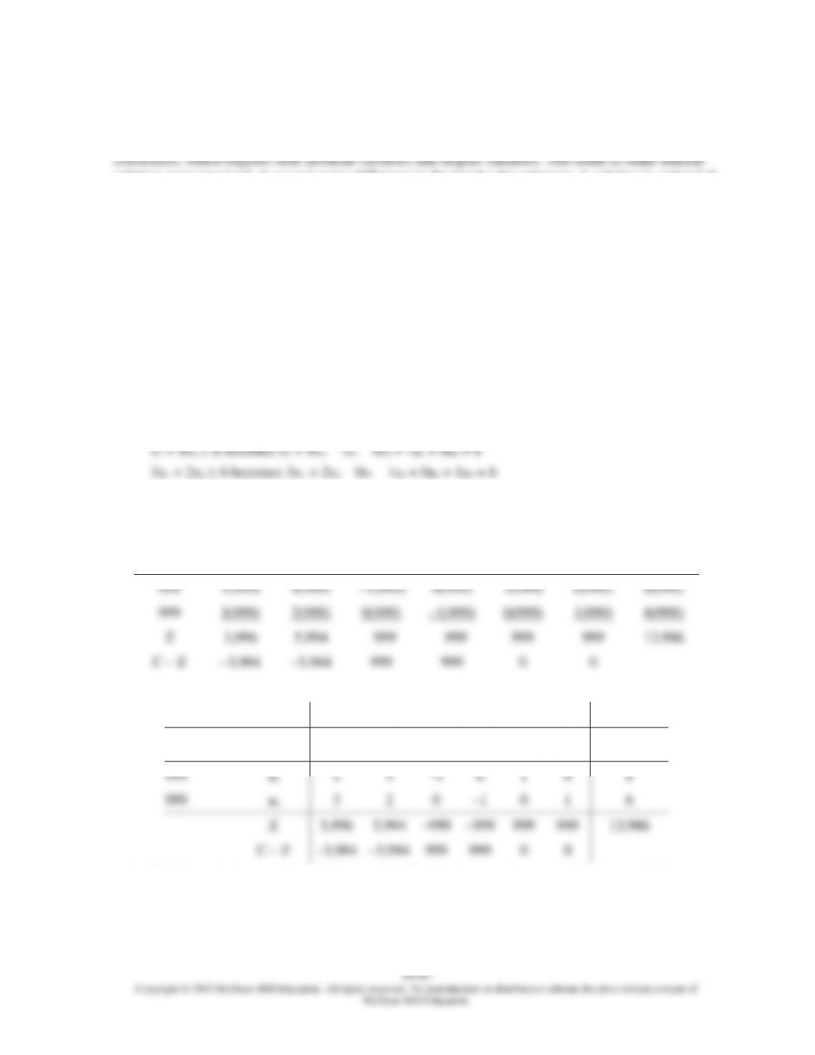
Solution to example
1. Rewrite the constraints so that they are in the proper form:
2. Rewrite the objective function (coefficients of C row):
12x1 + 10x2 + 0s1 + 0s2 + 999a1 + 999a2
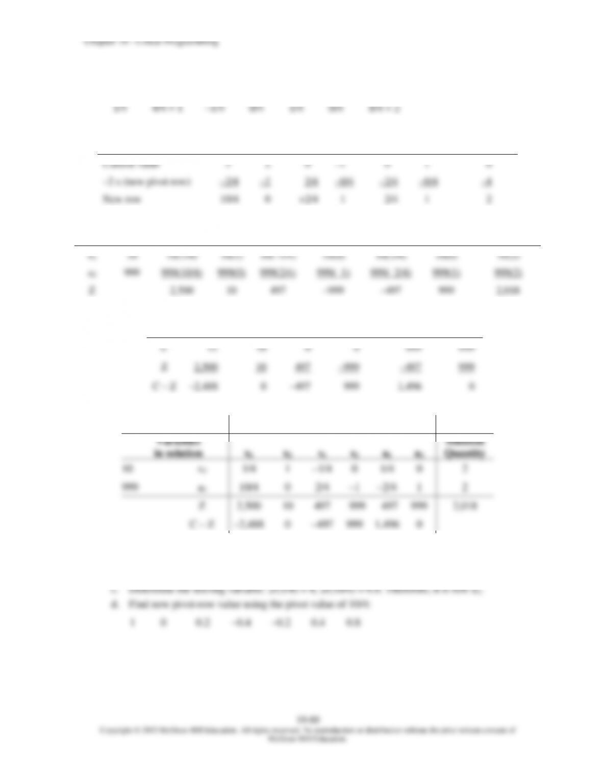
3. Compute values for rows Z and C – Z:
C
x1
x2
s1
s2
a1
a2
Quantity
999
1(999)
4(999)
–1(999)
0(999)
1(999)
0(999)
8(999)
999
3(999)
2(999)
0(999)
–1(999)
0(999)
1(999)
6(999)
Z
3,996
5,994
–999
–999
999
999
13,986
C – Z
–3,984
–5,984
999
999
0
0
4. Set up the initial tableau. (Note that the initial solution has all artificial variables.)
C
12
10
0
0
999
999
Variables
in solution
x1
x2
s1
s2
a1
a2
Solution
Quantity
999
a1
1
4
–1
0
1
0
8
999
a2
3
2
0
–1
0
1
6
Z
3,996
5,994
–999
–999
999
999
13,986
C – Z
–3,984
–5,984
999
999
0
0
5. Find the entering variable (largest negative C – Z value: x2 column) and leaving variable
(smaller of 8/4 = 2 and 6/2 =3; hence, row a1).