Chapter 19 – Linear Programming
19–71
Case: Custom Cabinets, Inc.
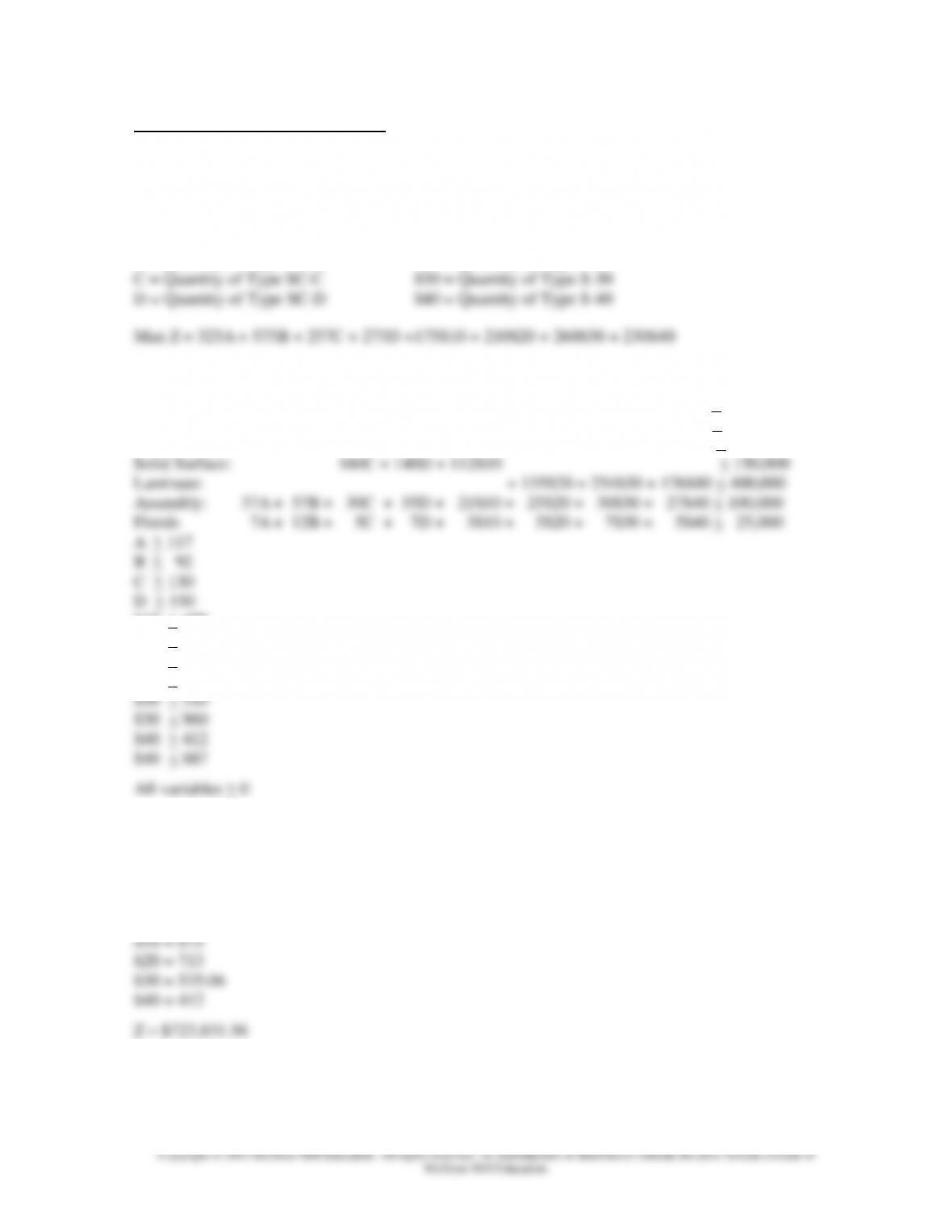
Problem Formulation:
Semi-custom Cabinets Standard Cabinets
A = Quantity of Type SC-A S10 = Quantity of Type S-10
B = Quantity of Type SC-B S20 = Quantity of Type S-20
Subject to:
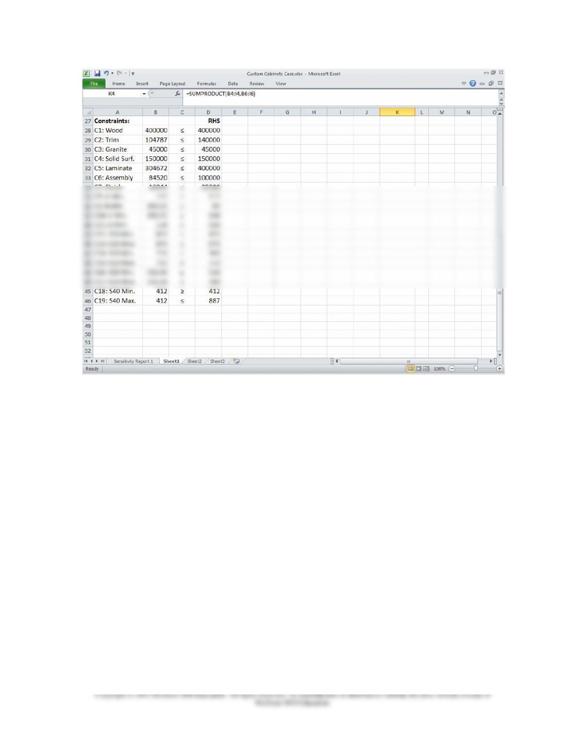
Wood: 125A + 160B + 140C + 200D + 60S10 + 110S20 + 200S30 + 180S40 < 400,000
Trim: 27A + 42B + 35C + 52D + 21S10 + 28S20 + 50S30 + 43S40 < 140,000
Granite: 175A + 243B < 45,000
S10 > 475
S10 < 875
S20 > 363
S20 < 713
Optimal Values
A = 117
B = 100.93
C = 193.75
D = 150
Chapter 19 – Linear Programming
Questions
1. In the given information in the case, we are told that workers could work 10% overtime in
Assembly and 5% overtime in Finishing. However, the C6: Assembly and C7: Finish
constraints both have slack and Shadow Prices equal to 0. Therefore, do not work overtime.
2. The C5: Laminate constraint also has slack and a shadow price of 0; therefore, do not purchase
additional laminate.
3. Wood has a shadow price of $1.30, and an allowable increase of 75,061.376 board feet.
4. The net profit in the initial solution is $723,831.56. The possible net profit when purchasing
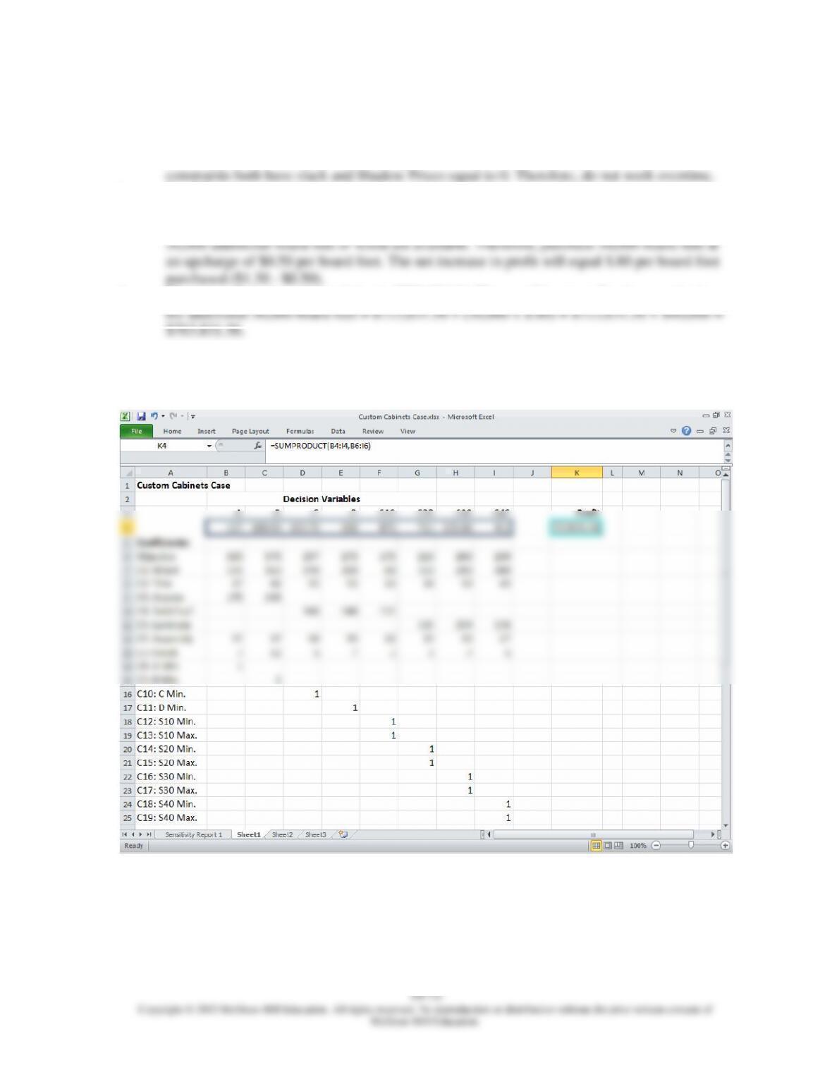
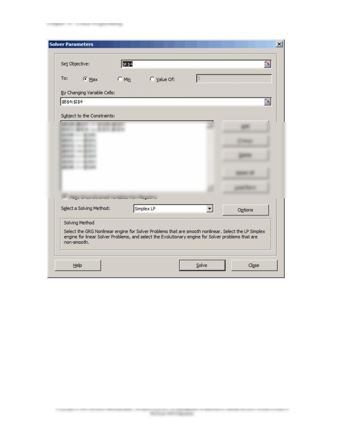
The Excel Solver solution and the Sensitivity Report are shown below. The Excel Solver solution is
shown in multiple screenshots.
Chapter 19 – Linear Programming
19–73
Chapter 19 – Linear Programming
19–74
Formulas used:
Cell
Formula
B28
=SUMPRODUCT(B$4:I$4,B7:I7)
B29
=SUMPRODUCT(B$4:I$4,B8:I8)
B30
=SUMPRODUCT(B$4:I$4,B9:I9)
B31
=SUMPRODUCT(B$4:I$4,B10:I10)
B32
=SUMPRODUCT(B$4:I$4,B11:I11)
B33
=SUMPRODUCT(B$4:I$4,B12:I12)
B34
=SUMPRODUCT(B$4:I$4,B13:I13)
B35
=SUMPRODUCT(B$4:I$4,B14:I14)
B36
=SUMPRODUCT(B$4:I$4,B15:I15)
B37
=SUMPRODUCT(B$4:I$4,B16:I16)
B38
=SUMPRODUCT(B$4:I$4,B17:I17)
B39
=SUMPRODUCT(B$4:I$4,B18:I18)
B40
=SUMPRODUCT(B$4:I$4,B19:I19)
B41
=SUMPRODUCT(B$4:I$4,B20:I20)
B42
=SUMPRODUCT(B$4:I$4,B21:I21)
B43
=SUMPRODUCT(B$4:I$4,B22:I22)
B44
=SUMPRODUCT(B$4:I$4,B23:I23)
B45
=SUMPRODUCT(B$4:I$4,B24:I24)
B46
=SUMPRODUCT(B$4:I$4,B25:I25)
K4
=SUMPRODUCT(B4:I4,B6:I6)
Note: The SUMPRODUCT formula was used to simplify entering constraints in the Solver model.
19–75
Chapter 19 – Linear Programming
19–76
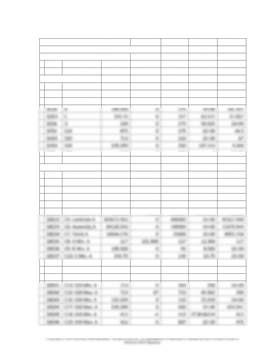
Sensitivity Report
Microsoft Excel 14.0 Sensitivity Report
Worksheet: [Custom Cabinets Case.xlsx]Sheet1
Report Created: 10/7/2013 11:53:05 AM
Variable Cells
Final
Reduced
Objective
Allowable
Allowable
Cell
Name
Value
Cost
Coefficient
Increase
Decrease
$B$4
A
117
0
325
101.800
1E+30
$C$4
B
100.926
0
575
1E+30
141.357
$D$4
C
193.75
0
257
63.571
57.857
$E$4
D
150
0
275
50.625
1E+30
$F$4
S10
875
0
175
1E+30
44.5
$G$4
S20
713
0
210
1E+30
67
$H$4
S30
535.059
0
260
107.143
4.444
$I$4
S40
412
0
230
4
1E+30
Constraints
Final
Shadow
Constraint
Allowable
Allowable
Cell
Name
Value
Price
R.H. Side
Increase
Decrease
$B$28
C1: Wood A
400000
1.3
400000
75061.376
5011.852
$B$29
C2: Trim A
104787.102
0
140000
1E+30
35212.898
$B$30
C3: Granite A
45000
1.510
45000
7611.75
2169
$B$31
C4: Solid Surf. A
150000
0.469
150000
5727.831
10200
$B$32
C5: Laminate A
304672.052
0
400000
1E+30
95327.948
$B$33
C6: Assembly A
84520.056
0
100000
1E+30
15479.944
$B$34
C7: Finish A
16044.276
0
25000
1E+30
8955.724
$B$35
C8: A Min. A
117
-101.800
117
12.394
117
$B$36
C9: B Min. A
100.926
0
92
8.926
1E+30
$B$37
C10: C Min. A
193.75
0
130
63.75
1E+30
$B$38
C11: D Min. A
150
-50.625
150
64.669
150
$B$39
C12: S10 Min. A
875
0
475
400
1E+30
$B$40
C13: S10 Max. A
875
44.5
875
91.071
131.891
$B$41
C14: S20 Min. A
713
0
363
350
1E+30
$B$42
C15: S20 Max. A
713
67
713
45.562
350
$B$43
C16: S30 Min. A
535.059
0
510
25.059
1E+30
$B$44
C17: S30 Max. A
535.059
0
960
1E+30
424.941
$B$45
C18: S40 Min. A
412
-4
412
27.8436214
412
$B$46
C19: S40 Max. A
412
0
887
1E+30
475
Chapter 19 – Linear Programming
19–77
Enrichment Module: The Simplex Method
The simplex method is a general-purpose linear-programming algorithm widely used to solve large-
scale problems. Although it lacks the intuitive appeal of the graphical approach, its ability to handle
problems with more than two decision variables makes it extremely valuable for solving problems
often encountered in operations management.
When teaching the simplex method, please consider the following points:
1. A computer package for simplex is highly desirable because it permits assigning a range of
problems and concentrating on interpretation of solutions rather than on technique.
taking place during computations, and gain some insight as to why.
3. Insight receives a boost when simplex and graphical solutions are compared for the same
problem.
4. Computations are best done without calculators; students should keep numbers in fractional
form.
5. Minimization, artificial variables, and ranging can be skipped without seriously impairing
appreciation and understanding of the simplex method.
The simplex technique involves a series of iterations; successive improvements are made until an
optimal solution is achieved. The technique requires simple mathematical operations (addition,
what is happening in the simplex calculations with a graphical solution to the problem.
Chapter 19 – Linear Programming
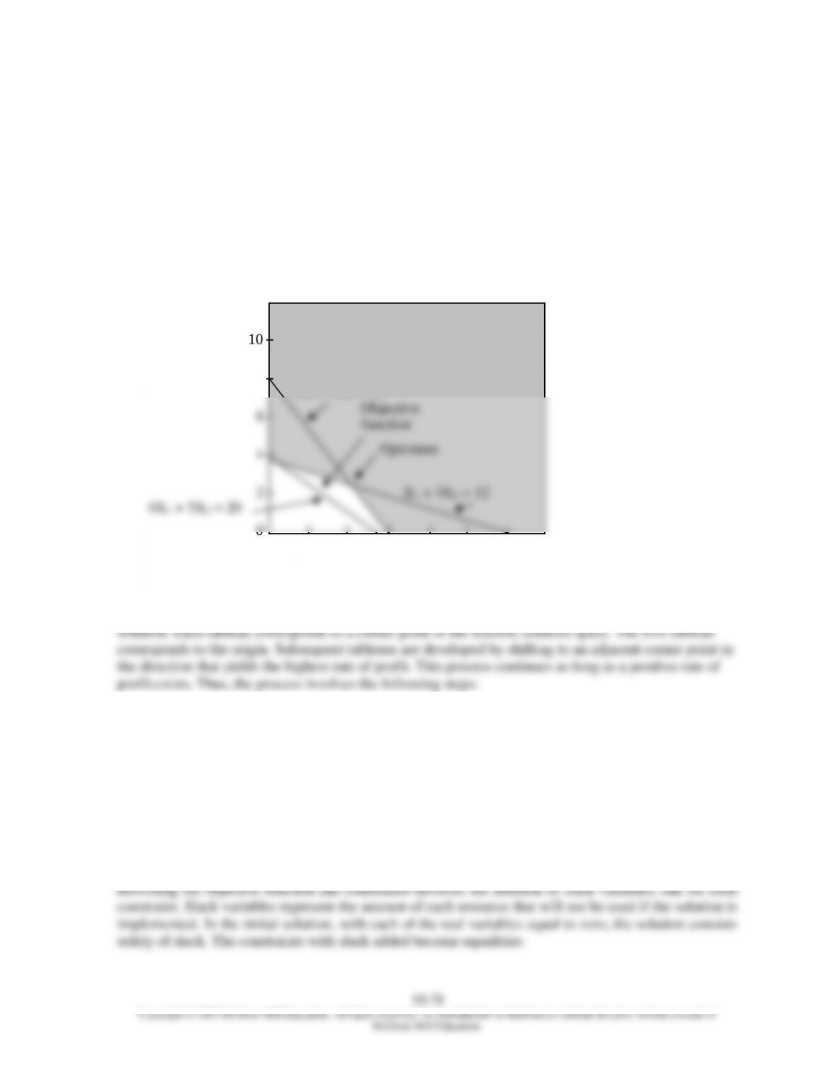
Let’s consider the simplex solution to the following problem:
Maximize
Z =
4x1
+ 5x2
Subject to
x1
+ 3x2
12
4x1
+ 3x2
24
x1, x2
0
The solution is shown graphically in Figure 1. Now let’s see how the simplex technique can be used to
obtain the solution.
Figure 1. Graphical Solution
The simplex technique involves generating a series of solutions in tabular form, called tableaus. By
inspecting the bottom row of each tableau, one can immediately tell if it represents the optimal
1. Set up the initial tableau.
2. Develop a revised tableau using the information contained in the first tableau.
3. Inspect to see if it is optimum.
4. Repeat steps 2 and 3 until no further improvement is possible.
Setting Up the Initial Tableau
Obtaining the initial tableau is a two-step process. First, we must rewrite the constraints to make them
equalities and modify the objective function slightly. Then we put this information into a table and
supply a few computations that are needed to complete the table.
X1
10
8
0
2 4 6 8 10 12
X2
4X1 + 3X2 = 24
Chapter 19 – Linear Programming
1)
x1
+ 3x2
+ 1s1
= 12
2)
4x1
+ 3x2
+ 1s2
= 24
1)
x1
+ 3x2
+ 1s1
+ 0s2
= 12
2)
4x1
+ 3x2
+ 0s1
+ 1s2
= 24
Z = 4x1 + 5x2 + 0s1 + 0s2
The slack variables are given coefficients of zero in the objective function because they do not
produce any contributions to profits. Thus, the information above can be summarized as:
Maximize Z = 4x1 + 5x2 + 0s1 + 0s2
Subject to
1)
x1
+ 3x2
+ 1s1
+ 0s2
= 12
2)
4x1
+ 3x2
+ 0s1
+ 1s2
= 24
added to the solution. The C – Z row shows the potential for increasing profit if one unit of the
variable in that column were added to the solution.
To compute the Z values, multiply the coefficients in each column by their respective row profit per
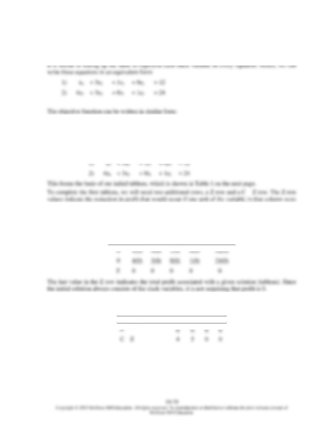
unit amounts, and sum within columns. To begin with, all values are zero:
C
x1
x2
s1
s2
Quantity
0
1(0)
3(0)
1(0)
0(0)
12(0)
0
4(0)
3(0)
0(0)
1(0)
24(0)
Z
0
0
0
0
0
The last value in the Z row indicates the total profit associated with a given solution (tableau). Since
the initial solution always consists of the slack variables, it is not surprising that profit is 0.
Values in the C – Z row are computed by subtracting the Z value in each column from the value of the
objective row for that column. Thus,
Variable row
x1
x2
s1
s2
Objective row (C)
4
5
0
0
Z
0
0
0
0
C – Z
4
5
0
0
Chapter 19 – Linear Programming
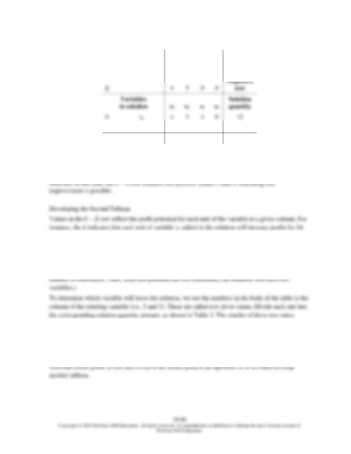
Table 1 Partial Initial Tableau
Profit per unit
for variables
in solution
Decision
Variables
C
4
5
0
0
Objective
row
Variables
in solution
x1
x2
s1
s2
Solution
quantity
0
s1
1
3
1
0
12
0
s2
4
3
0
1
24
The completed tableau is shown in Table 2.
The Test for Optimality
If all the values in the C – Z row of any tableau are zero or negative, the optimal solution has been
Similarly, the 5 indicates that each unit of x2 will contribute $5 to profits. Given a choice between $4
per unit and $5 per unit, we select the larger and focus on that column, which means that x2 will come
into the solution. Now we must determine which variable will leave the solution. (At each tableau, one
variable will come into the solution, and one will go out of solution, keeping the number of variables
in the solution constant. Note that the number of variables in the solution must always equal the
indicates the variable that will leave the solution. Thus, variable s1 will leave and be replaced with x2.
In graphical terms, we have moved up the x2 axis to the next corner point. By determining the smallest
ratio, we have found which constraint is the most limiting. In Figure 1, note that the two constraints
intersect the x2 axis at 4 and 8, the two row ratios we have just computed. The second tableau will
describe the corner point where x2 = 4 and x1 = 0; it will indicate the profits and quantities associated