Chapter 19 – Linear Programming
19–41
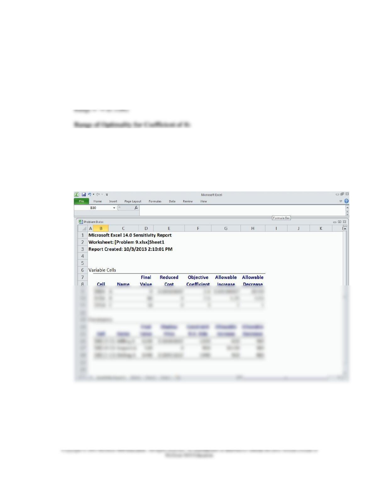
Determine the range of optimality for the three coefficients of the objective function.
To determine the range of optimality for each coefficient, we must use the following values
found under Variable Cells in the Sensitivity Report:
Objective Coefficient, Allowable Increase, and Allowable Decrease.
Range of Optimality for Coefficient of A:
2.4 – 1E+30 and 2.4 + 0.642
2.5 – 0.55 and 2.5+ 1.25
Range = 1.95 to 3.75
Range of Optimality for Coefficient of C:
3 – 1 and 3 + 2
Range = 2 to 5
The Sensitivity Report is shown below:
19–42
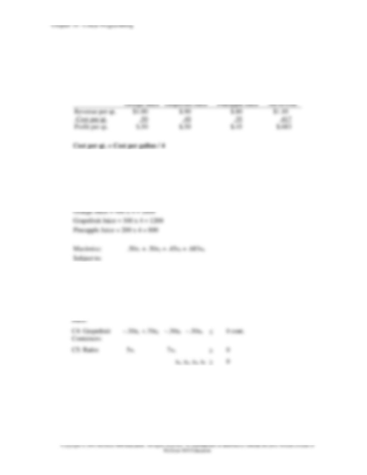
10. Formulate the model:
x1 = number of one-quart containers of orange juice
x2 = number of one-quart containers of grapefruit juice
x3 = number of one-quart containers of pineapple juice
x4 = number of one-quart containers of All-in-One
Orange Juice
Grapefruit Juice
Pineapple Juice
All-in–One
Revenue per qt.
$1.00
$.90
$.80
$1.10
-Cost per qt.
.50
.40
.35
.417
Profit per qt.
$.50
$.50
$.45
$.683
Cost per qt. = Cost per gallon / 4
Orange Juice = $2.00 / 4 = $.50
Grapefruit Juice = $1.60 / 4 = $.40
Pineapple Juice = $1.40 / 4 = $.35
All-in–One = [$.50 +$.40 + $.35] / 3 = $.417
Quarts On Hand = Gallons On Hand x 4
C1 Orange
Juice:
1x1
+.333x4
1600 qt.
C2: Grapefruit
Juice:
1x2
+.333x4
1200 qt.
C3: Pineapple
Juice:
1x3
+.333x4
800 qt.
C4: Grapefruit
Containers:
–.30x1
+.70x2
–.30x3
–.30x4
0 cont.
C5: Ratio:
5x1
–7x3
0
x1, x2, x3, x4
0
Chapter 19 – Linear Programming
19–43
Notes on constraint development:
C5: The ratio of the number of containers of orange juice (x1) to the number of containers
of pineapple juice (x3) should be at least 7 to 5.
�
�
5x1 ≥ 7x3
5x1 – 7x3 ≥ 0
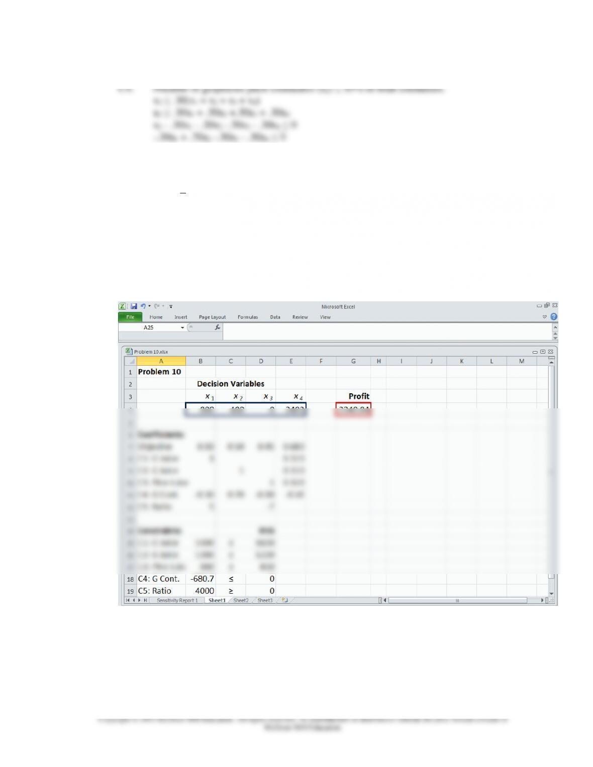
The optimal values of the decision variables are: x1 = 800, x2 = 400, x3 = 0, x4 = 2402. The
optimal value of the objective function coefficient is Z = 2240.84.
Refer to the Excel Solver solution below:
Chapter 19 – Linear Programming
19–44
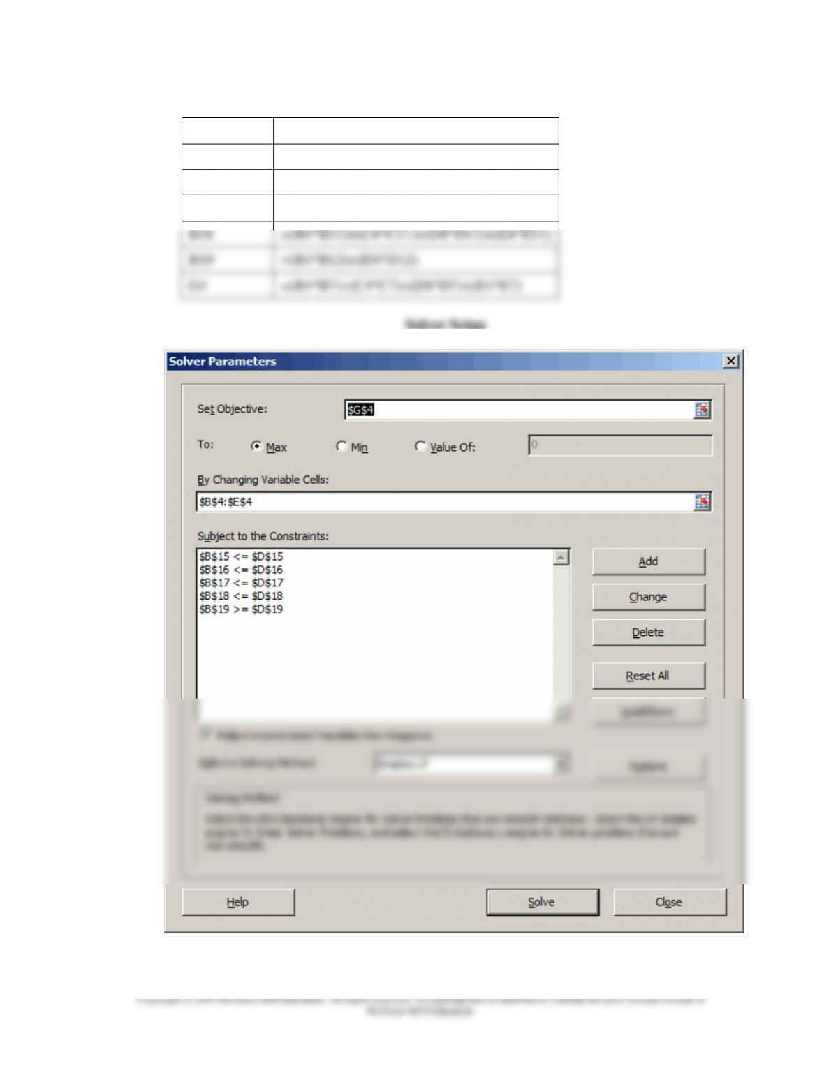
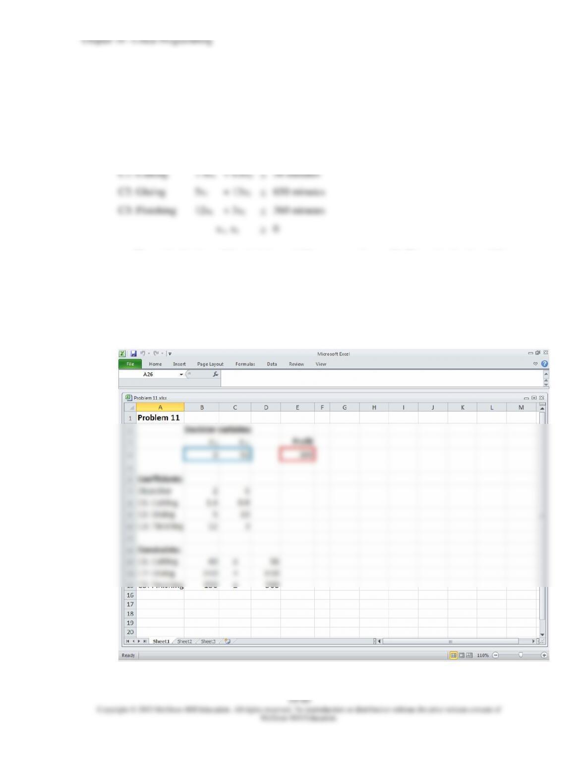
Formulas used:
Cell
Formula
B15
=(B4*B8)+(E4*E8)
B16
=(C4*C9)+(E4*E9)
B17
=(D4*D10)+(E4*E10)
B18
=(B4*B11)+(C4*C11)+(D4*D11)+(E4*E11)
B19
=(B4*B12)+(D4*D12)
G4
=(B4*B7)+(C4*C7)+(D4*D7)+(E4*E7)
Chapter 19 – Linear Programming
19–46
Formulas used:
Cell
Formula
B13
=(B$4*B8)+(C$4*C8)
B14
=(B$4*B9)+(C$4*C9)
B15
=(B$4*B10)+(C$4*C10)
E4
=(B4*B7)+(C4*C7)
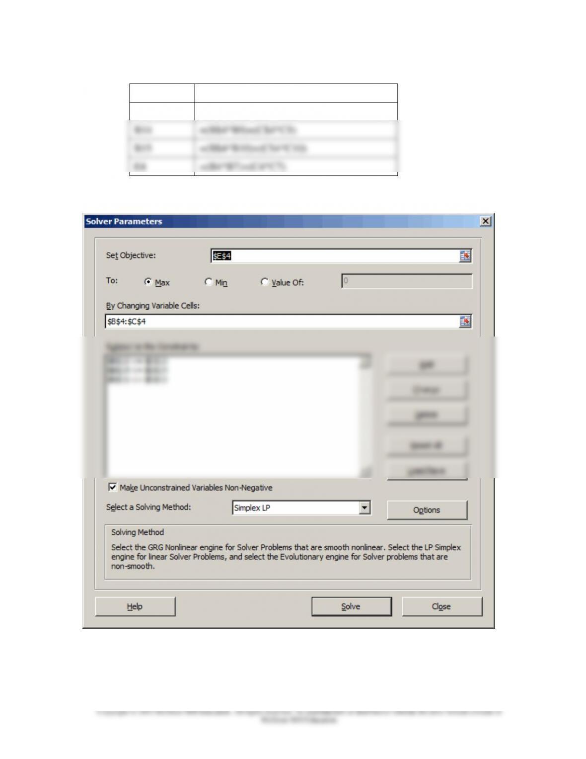
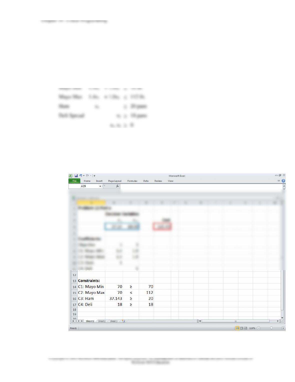
Solver Setup
19–47
12. Formulate the model:
x1 = pans of ham spread to make
x2 = pans of deli spread to make
Maximize
2x1
+ 4x2
(Profit) or Minimize 3x1 + 3x2 (Cost)
Subject to:
Mayo Min
1.4x1
+ 1.0x2
70 lb.
Mayo Max
1.4x1
+ 1.0x2
112 lb.
Ham
x1
20 pans
Deli Spread
x2
18 pans
x1, x2
0
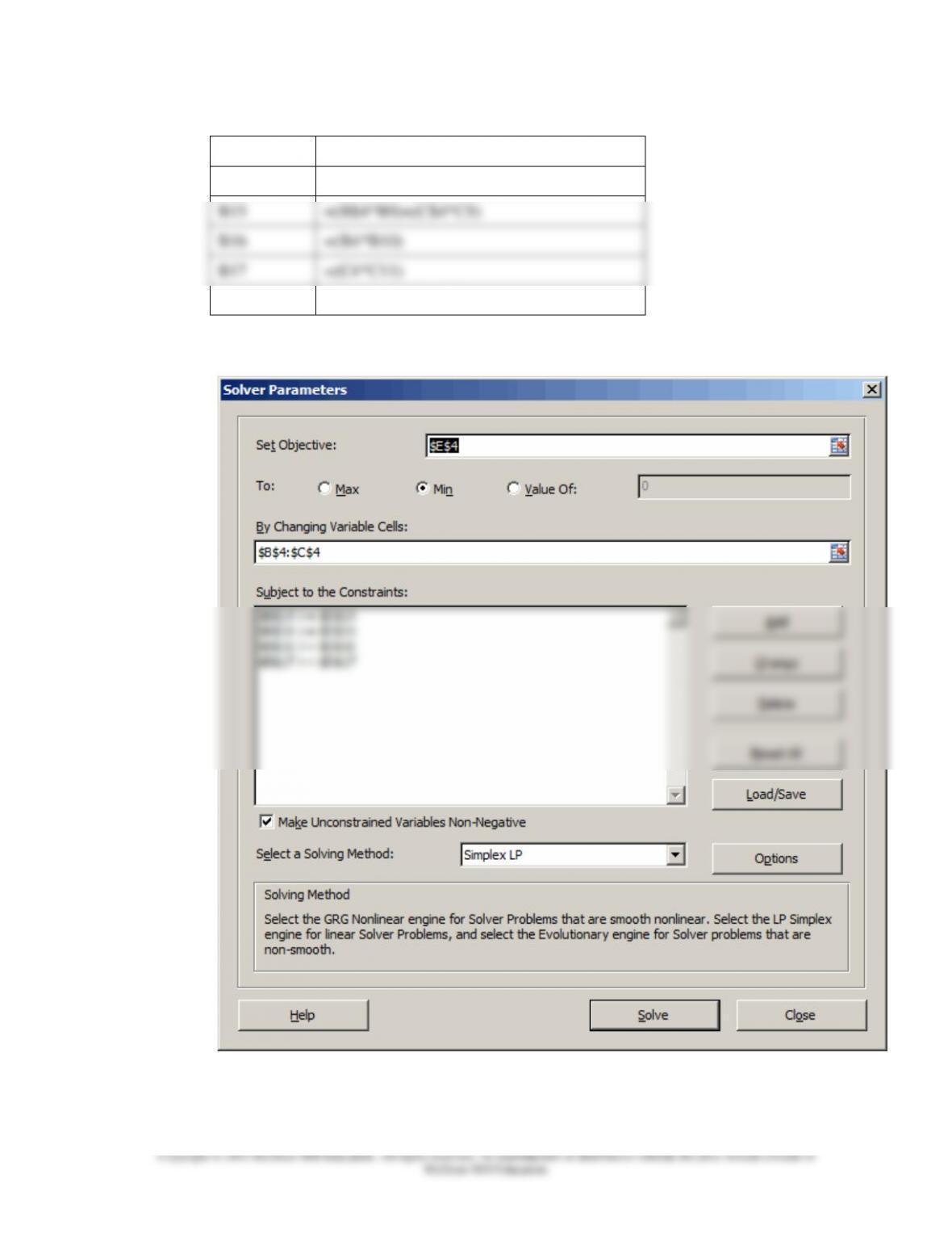
a. Determine the solution that will minimize cost.
The optimal values of the decision variables are: x1 = 37.14, x2 = 18. The optimal value of
the objective function coefficient is Z = $165.43 (cost).
The Excel Solver solution for the minimization problem is shown below:
Chapter 19 – Linear Programming
19–48
Formulas used:
Cell
Formula
B14
=(B$4*B8)+(C$4*C8)
B15
=(B$4*B9)+(C$4*C9)
B16
=(B4*B10)
B17
=(C4*C11)
E4
=(B4*B7)+(C4*C7)
Solver Setup
19–49
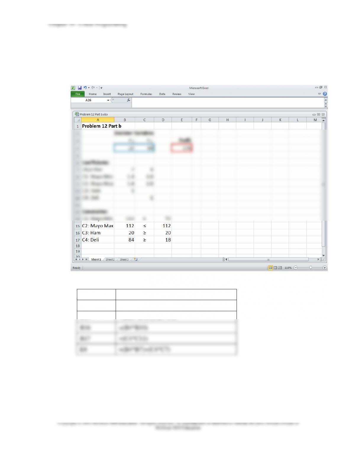
b. Determine the solution that will maximize profit.
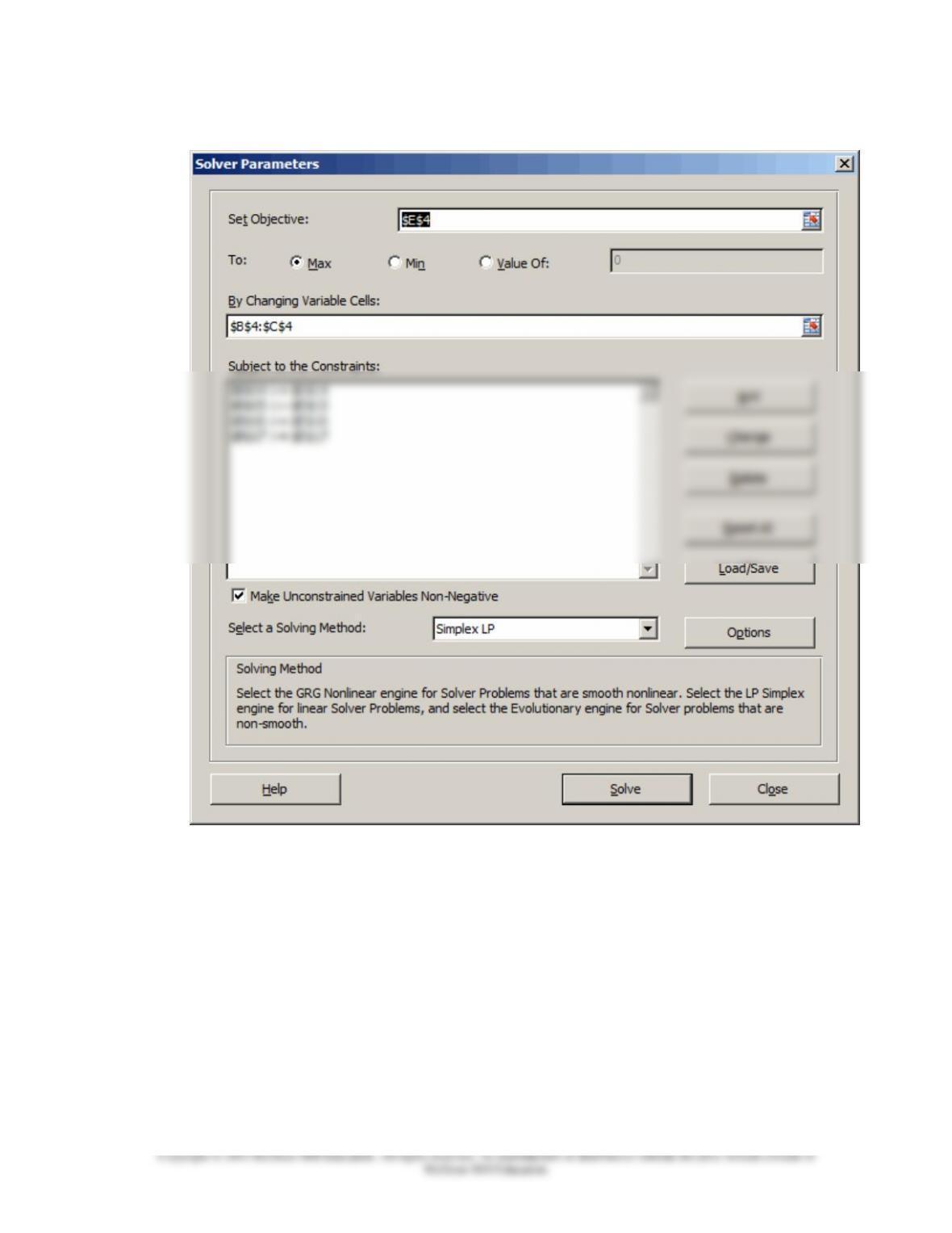
The optimal values of the decision variables are: x1 = 20, x2 = 84. The optimal value of the
objective function coefficient is Z = $376 (profit).
The Excel Solver solution for the maximization problem is shown below:
Formulas used:
Cell
Formula
B14
=(B$4*B8)+(C$4*C8)
B15
=(B$4*B9)+(C$4*C9)
B16
=(B4*B10)
B17
=(C4*C11)
E4
=(B4*B7)+(C4*C7)
Chapter 19 – Linear Programming
19–50
Solver Setup