Chapter 19 – Linear Programming
19-1
CHAPTER 19
LINEAR PROGRAMMING
Teaching Notes
The main goal of this supplement is to provide students with an overview of the types of problems that
have been solved using linear programming (LP). In the process of learning the different types of
problems that can be solved with LP, students also must develop a very basic understanding of the
assumptions and special features of LP problems.
Students also should learn the basics of developing and formulating linear programming models for
simple problems, solve two-variable linear programming problems by the graphical procedure, and
interpret the resulting outcome. In the process of solving these graphical problems, we must stress the
role and importance of extreme points in obtaining an optimal solution.
Improvements in computer hardware and software technology and the popularity of the software
package Microsoft Excel make the use of computers in solving linear programming problems
accessible to many users. Therefore, a main goal of the chapter should be to allow students to solve
linear programming problems using Excel. More importantly, we need to ensure that students are able
to interpret the results obtained from Excel or any another computer software package.
Answers to Discussion and Review Questions
1. Linear programming is well-suited to constrained optimization problems that satisfy the
following assumptions:
2. The “area of feasibility,” or feasible solution space is the set of all combinations of values of
3. Redundant constraints do not affect the feasible region for a linear programming problem.
4. An iso-cost line represents the set of all possible combinations of two input decision variables
5. Sliding an objective function line towards the origin represents a decrease in its value (i.e.,
6. a. Basic variable: In a linear programming solution, it is a variable not equal to zero.
b. Shadow price: It is the change in the value of the objective function for a one-unit change
in the right-hand-side value of a constraint.
Chapter 19 – Linear Programming
19-2
Solution to Problems
1. a. Graph the constraints and the objective function:
Material constraint:
6x1 + 4x2 ≤ 48
Replace the inequality sign with an equal sign:
6x1 + 4(0) = 48
6x1 = 48
x1 = 8
A second point on the line is (8, 0).
4(0) + 8x2 = 80
8x2 = 80
x2 = 10
One point on the line is (0, 10).
Set x2 = 0 and solve for x1:
Let 4x1 + 3x2 = 24.
Set x1 = 0 and solve for x2:
4(0) + 3x2 = 24
3x2 = 24
x2 = 8
A second point on the line is (6, 0).
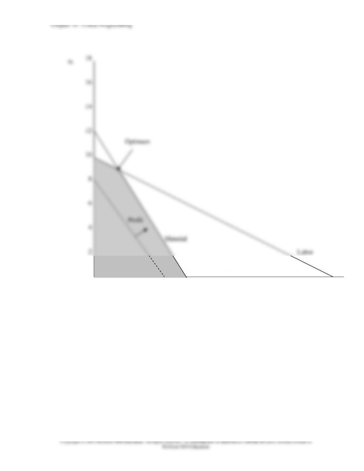
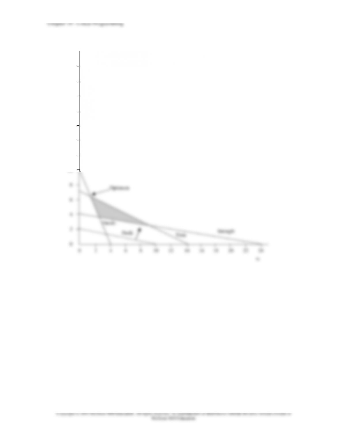
The graph and the feasible solution space (shaded) are shown below:
19-3
Optimum
Labor
Material
x2
18
16
14
12
10
8
6
4
2
Profit
2 4 6 8 10 12 14 16 18 20
x1
Chapter 19 – Linear Programming
19-4
(1) As we slide the profit line away from the origin, we reach the optimum point indicated
in the graph above (at the intersection of the two constraints). The optimal values of
the decision variables are x1 = 2, x2 = 9, and the optimal objective function value = Z =
35. The work for these solutions is shown below:
Simultaneous solution:
Material: 6x1 + 4x2 = 48
Labor: 4x1 + 8x2 = 80
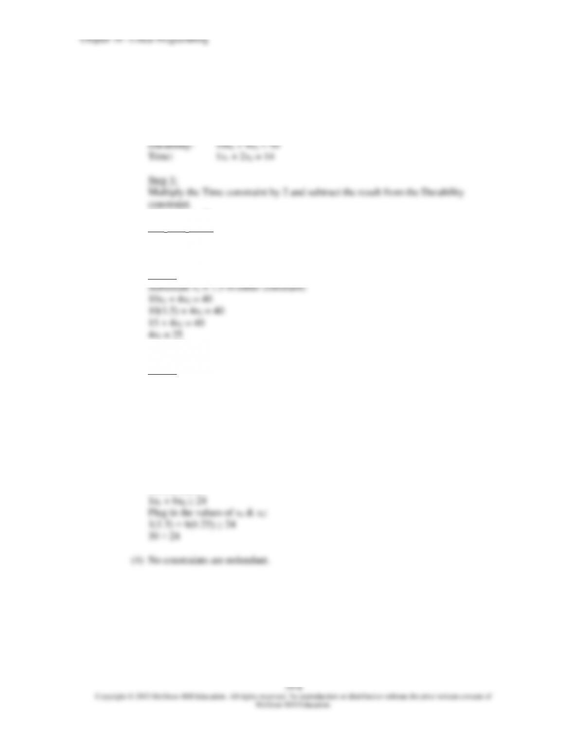
Step 1:
Multiply the Material constraint by 2 and subtract the Labor constraint from the result.
Step 2:
Substitute x1 = 2 in either constraint:
6x1 + 4x2 = 48
Step 3:
Substitute the values of x1 and x2 in the objective function:
(2) No constraints have slack. Both ≤ constraints are binding.
(3) No constraints have surplus. There are no ≥ constraints.
(4) No constraints are redundant.
Chapter 19 – Linear Programming
19-5
b. Graph the constraints and the objective function:
Durability constraint:
10x1 + 4x2 ≥ 40
Replace the inequality sign with an equal sign:
10x1 + 4(0) = 40
10x1 = 40
x1 = 4
A second point on the line is (4, 0).
Strength constraint:
1x1 + 6x2 ≥ 24
Replace the inequality sign with an equal sign:
1x1 + 6(0) = 24
x1 = 24
A second point on the line is (24, 0).
19-6
Time constraint:
1x1 + 2x2 ≤ 14
Replace the inequality sign with an equal sign:
1x1 + 2x2 = 14
Set x1 = 0 and solve for x2:
1x1 + 2(0) = 14
x1 = 14
A second point on the line is (14, 0).
Objective function:
Let 2x1 + 10x2 = 20.
Set x1 = 0 and solve for x2:
2(0) + 10x2 = 20
10x2 = 20
x2 = 2
The graph and the feasible solution space (shaded) are shown below:
x2
Optimum
24
22
20
18
16
14
12
10
8
6
4
2
0
0 2 4 6 8 10 12 14 16 18 20 22 24
Strength
Time
Durab.
x1
Profit
Chapter 19 – Linear Programming
19-9
c. Graph the constraints and the objective function:
Material constraint:
20A + 6B ≤ 600
Replace the inequality sign with an equal sign:
20A + 6B = 600
20A + 6(0) = 600
20A = 600
A = 30
A second point on the line is (30, 0).
Machinery constraint:
25A + 20B ≤ 1,000
Replace the inequality sign with an equal sign:
25A + 20B = 1,000
Set A = 0 and solve for B:
25(0) + 20B = 1,000
Chapter 19 – Linear Programming
19–10
Labor constraint:
20A + 30B ≤ 1,200
Replace the inequality sign with an equal sign:
One point on the line is (0, 40).
Set B = 0 and solve for A:
20A + 30(0) = 1,200
20A = 1,200
A = 60
A second point on the line is (60, 0).
Objective function:
Let 6A + 3B = 120.
Set A = 0 and solve for B:
6(0) + 3B = 120
3B = 120
The graph and the feasible solution space (shaded) are shown below: