Chapter 18 – Management of Waiting Lines
18–11
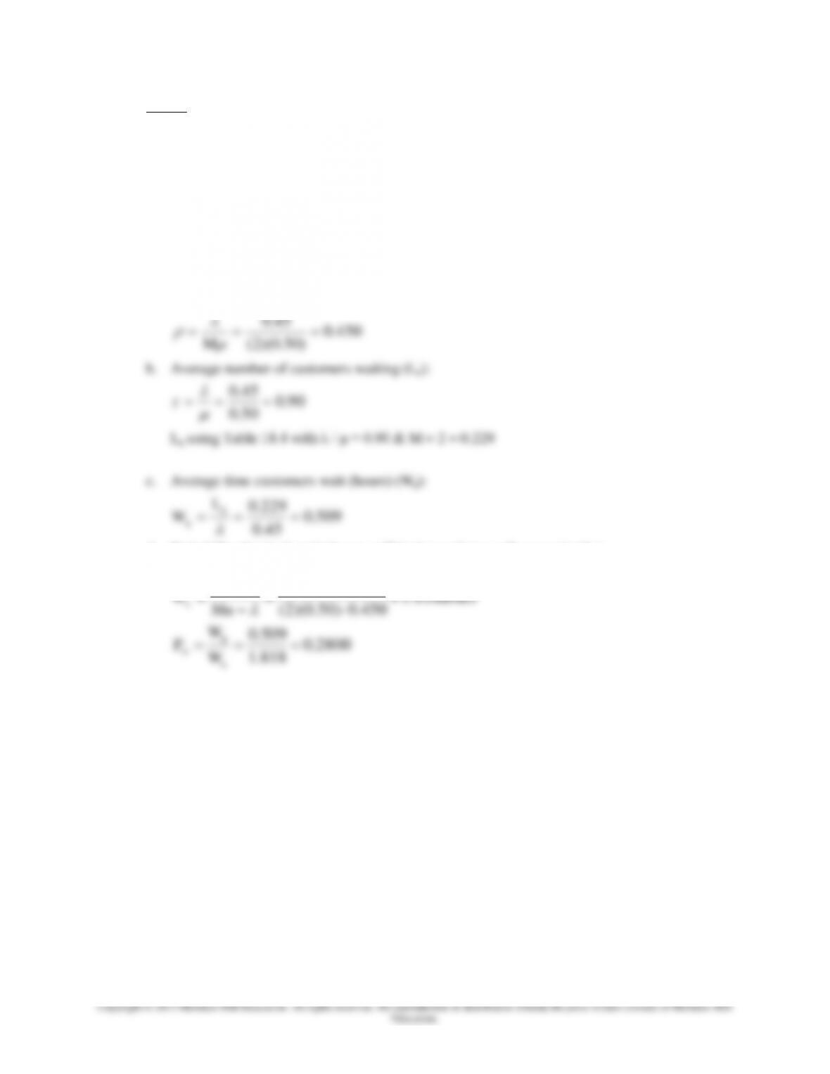
5. Given:
= 0.45 calls/hour (Poisson)
Mean service time = 2 hours/call (exponentially distributed)
M = 2 ambulances
[Multiple Servers, M/M/S]
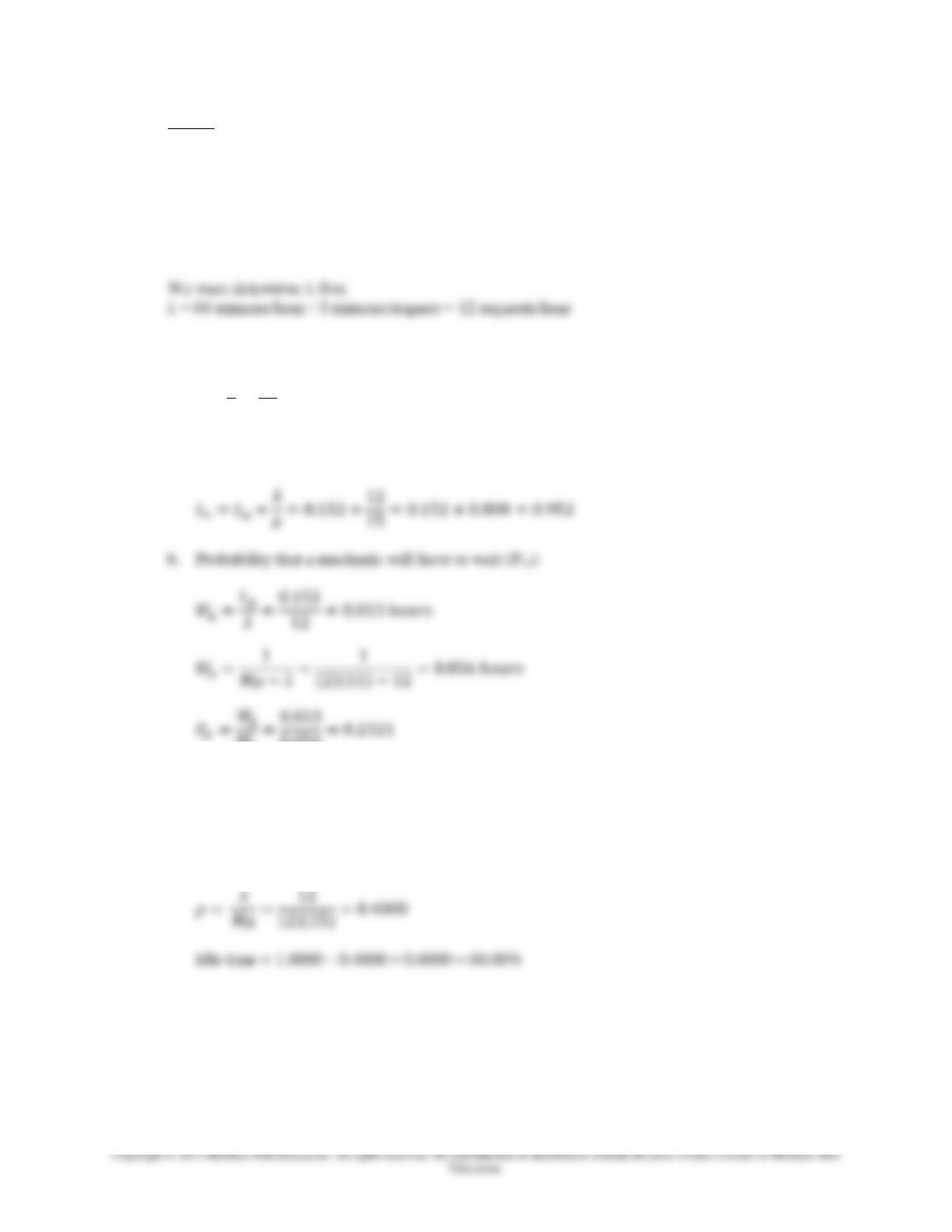
We must determine first (we will use hours)μ
= 1 call/2 hours = 0.5 calls/hour
a. System utilization (ρ):
450.0
)50.0)(2(
45.0
M
b. Average number of customers waiting (Lq):
90.0
50.0
45.0
r
Lq using Table 18.4 with / = 0.λ0 & M = 2 = 0.229
c. Average time customers wait (hours) (Wq):
509.0
0.45
229.0
q
q
L
W
d. Probability that both ambulances will be busy when a call comes in (Pw):
hours1.818
0.450– (2)(0.50)
11
Mu
Wa
2800.0
818.1
509.0
a
q
wW
W
P
18–12
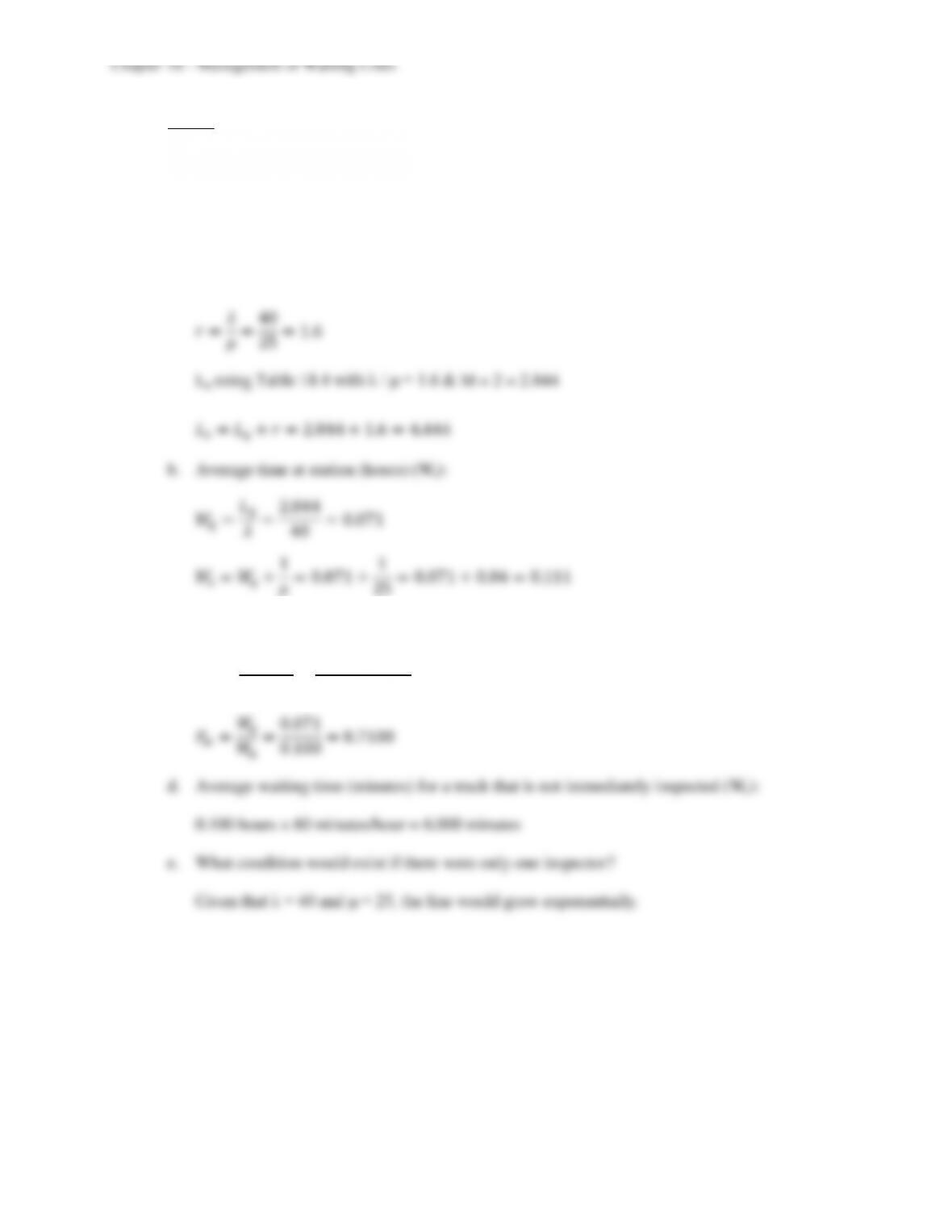
6. Given:
= 40 trucks/hour (Poisson)
= 25 trucks/hour (Poisson)
M = 2
[Multiple Servers, M/M/S]
a. Average number of trucks waiting plus being inspected (Ls):
c. Probability that both inspectors are busy (Pw):
Chapter 18 – Management of Waiting Lines
18–13
Education.
f. Maximum line length (Lmax) for a probability of 97%:
= 40, = 25, M = 2, Lq = 2.844, r = 1.6
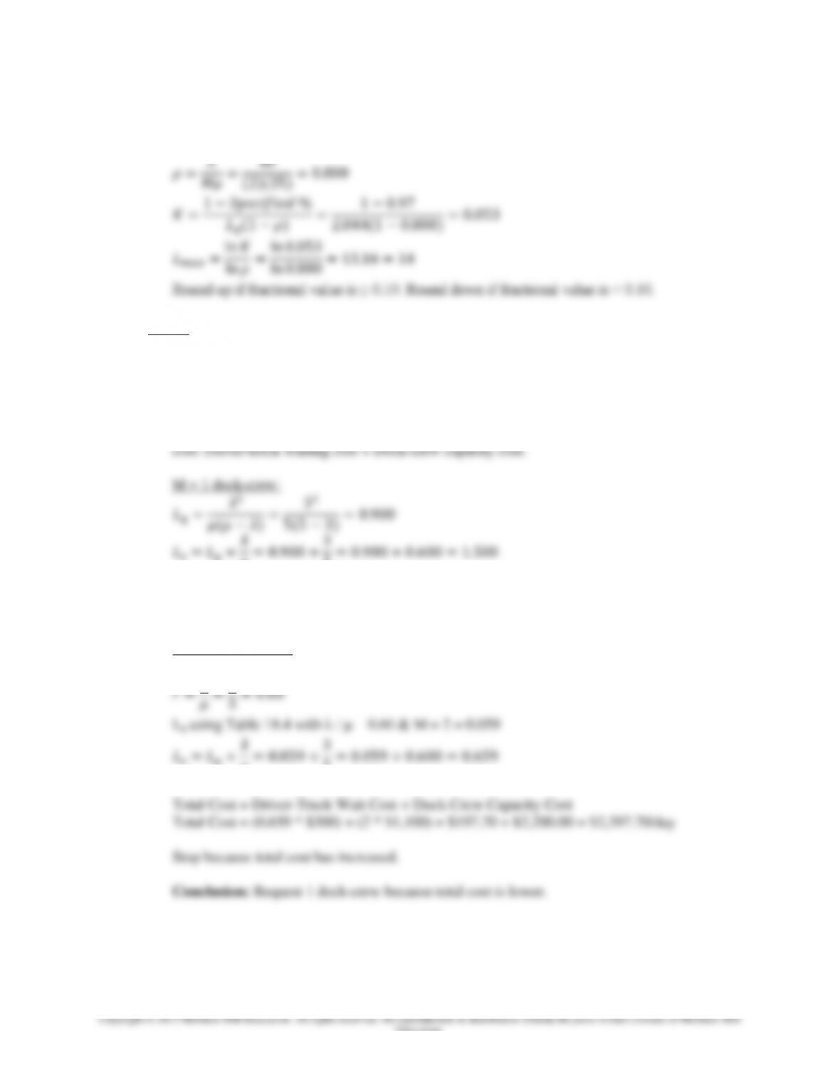
7. Given:
Cost of each driver-truck combination = $300 per day.
Cost of each dock-crew = $1,100 per day.
a. If = 3/day (Poisson) and = 5/day (Poisson), how many docks should be requested?
To solve this we need to experiment with different values and observe what happens to total
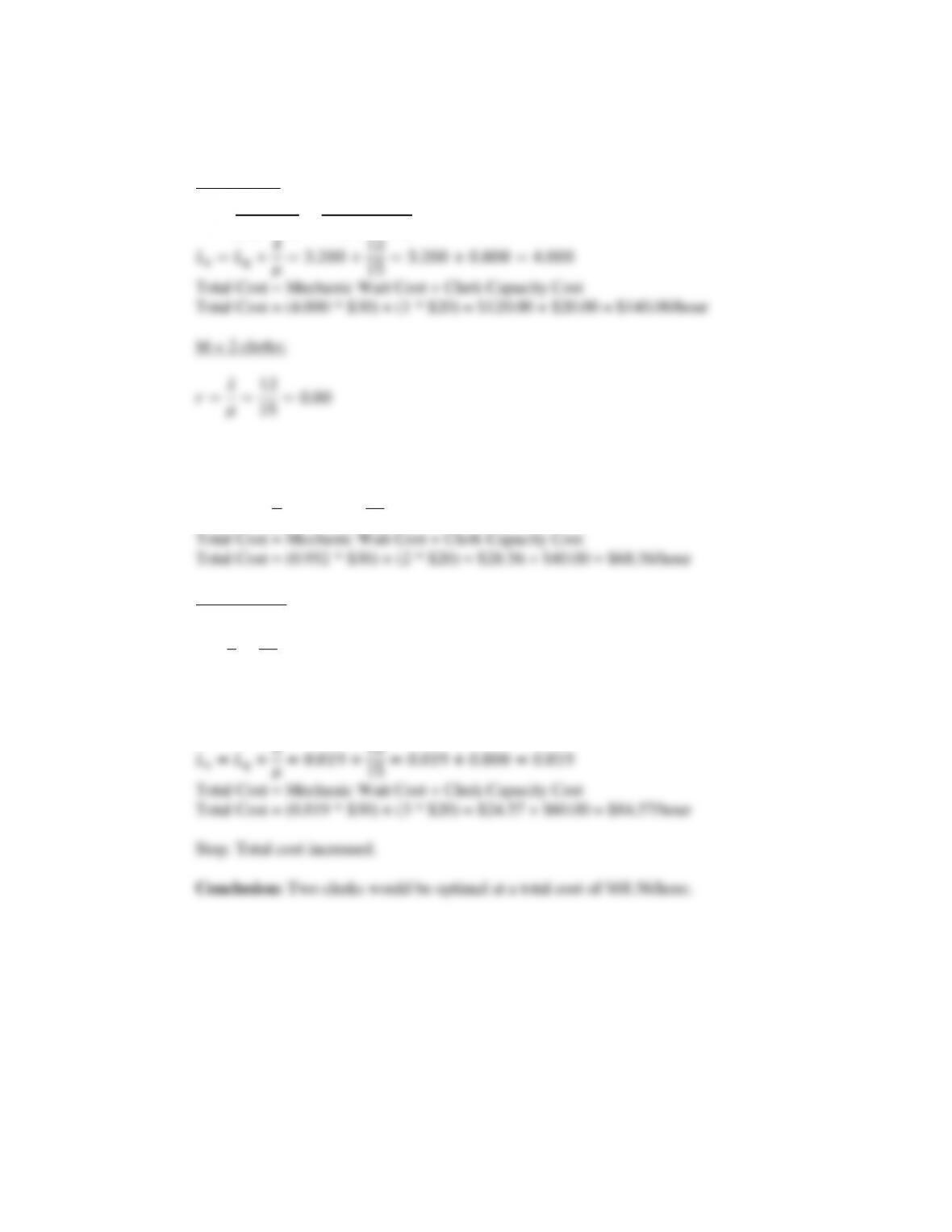
Total Cost = Driver-Truck Wait Cost + Dock-Crew Capacity Cost
Total Cost = (1.500 * $300) + (1 * $1,100) = $450.00 + $1,100.00 = $1,550.00/day
M = 2 docks-crews:
18–14
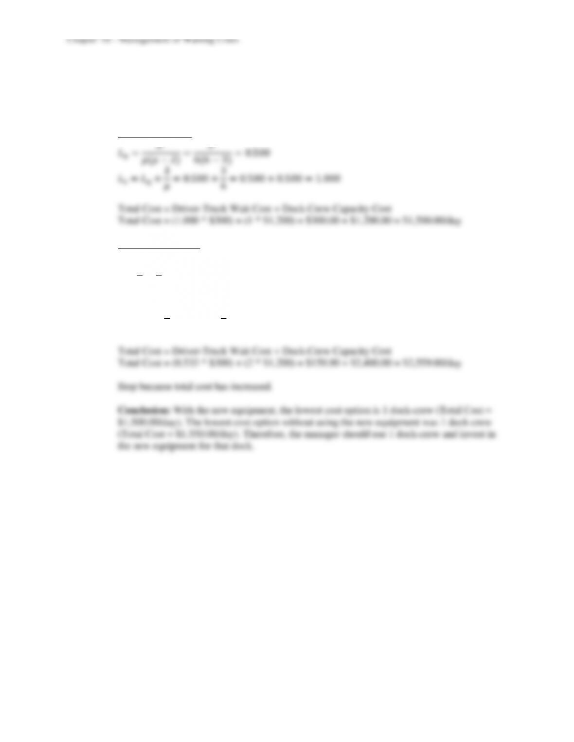
b. New equipment would cost $100 per day for each dock and would increase to 6/day.
Cost of each driver-truck combination = $300 per day.
Cost of each dock-crew + new equipment = $1,100 + $100 = $1,200 per day.
M = 1 dock-crew:
M = 2 docks-crews:
Lq using Table 18.4 with / = 0.50 & M = 2 = 0.033
Chapter 18 – Management of Waiting Lines
18–15
8. Given:
Time between requests can be modeled by a negative exponential distribution that has a mean = 5
minutes.
= 15 requests/hour
M = 2
[Multiple Servers, M/M/S]
a. Average number of mechanics at the counter, including those being served (Ls):
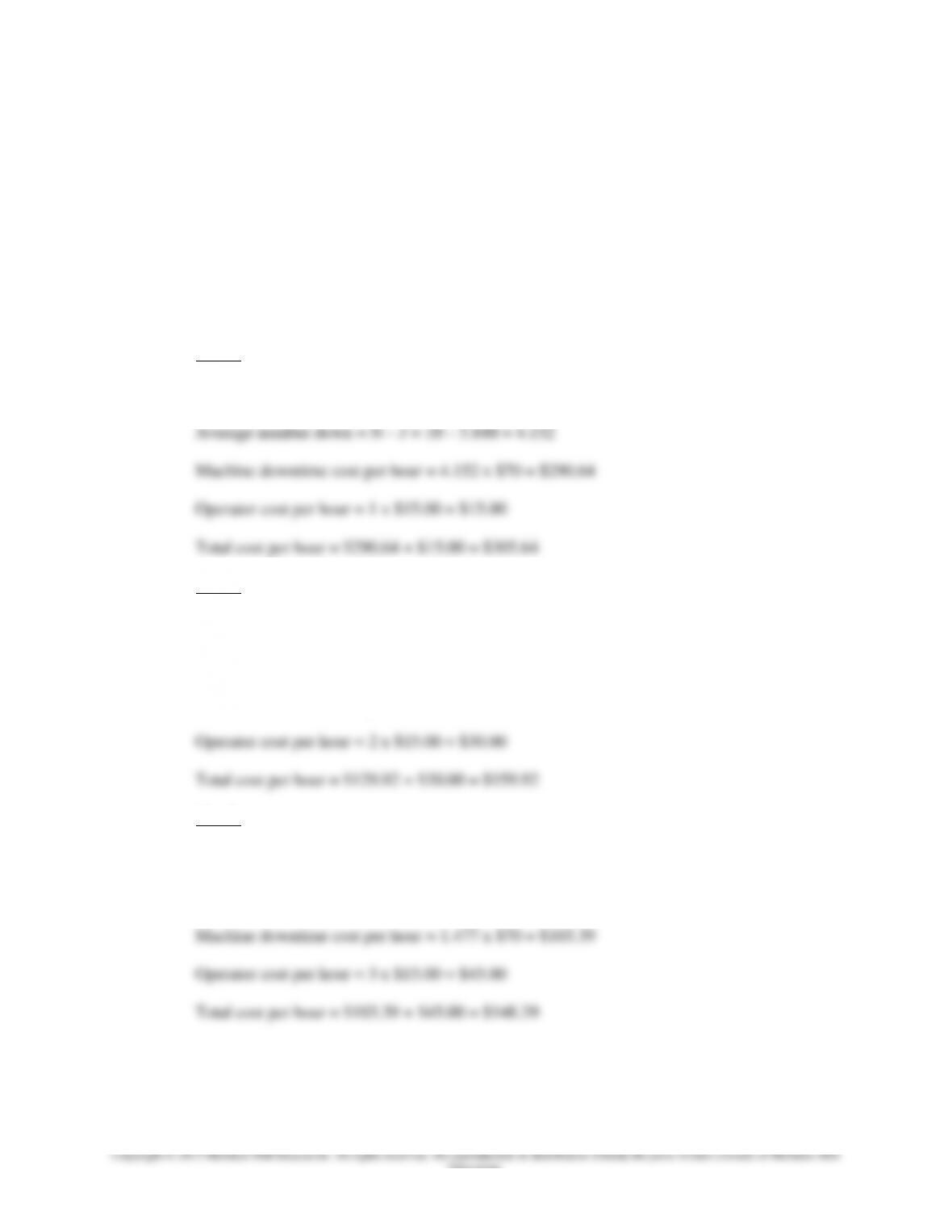
Lq using Table 18.4 with / = 0.80 & M = 2 = 0.152
c. If a mechanic has to wait, how long will the wait be (Wa)?
From Part b: 0.056 hours
d. Percentage of idle time (carry % to two decimals):
Chapter 18 – Management of Waiting Lines
18–16
e. Clerks cost $20/hour & mechanics cost $30/hour. Determine the number of clerks to
minimize total cost:
M = 1 clerk:
Lq using Table 18.4 with / = 0.80 & M = 2 = 0.152
M = 3 clerks:
Lq using Table 18.4 with / = 0.80 & M = 3 = 0.019
Chapter 18 – Management of Waiting Lines
9. Given:
N = 5 customers
T = 1 day
U = 4 days
M = 1 field rep
[Finite–source queuing model]
a. Expected number of customers waiting (L):
b. Average Wait Time (W) + Average Service Time (T):
W + T = 1.242 days + 1 day = 2.242 days
c. Percentage idle time:
18–18
10. Given:
N = 10 machines
T = 14 minutes
U = 86 minutes
M = 2 operators
[Finite–source queuing model]
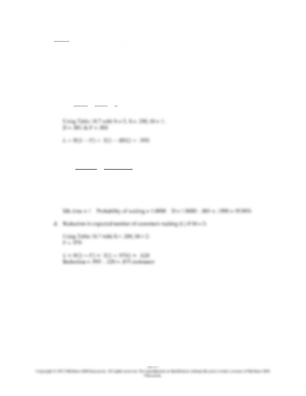
a. Probability that a machine will have to wait for an adjustment (D):
Probability of waiting = D = .4370
b. Average number of machines waiting (L):
d. Expected hourly output of each machine, taking adjustments into account:
Expected hourly output per machine = Percentage time machine is running x Output while
running
Chapter 18 – Management of Waiting Lines
18–19
Education.
e. Machine downtime cost = $70/hour & Operator cost = $15/hour. Determine the optimum
number of operators:
Machine downtime cost per hour = Average number down x Machine downtime cost per
hour
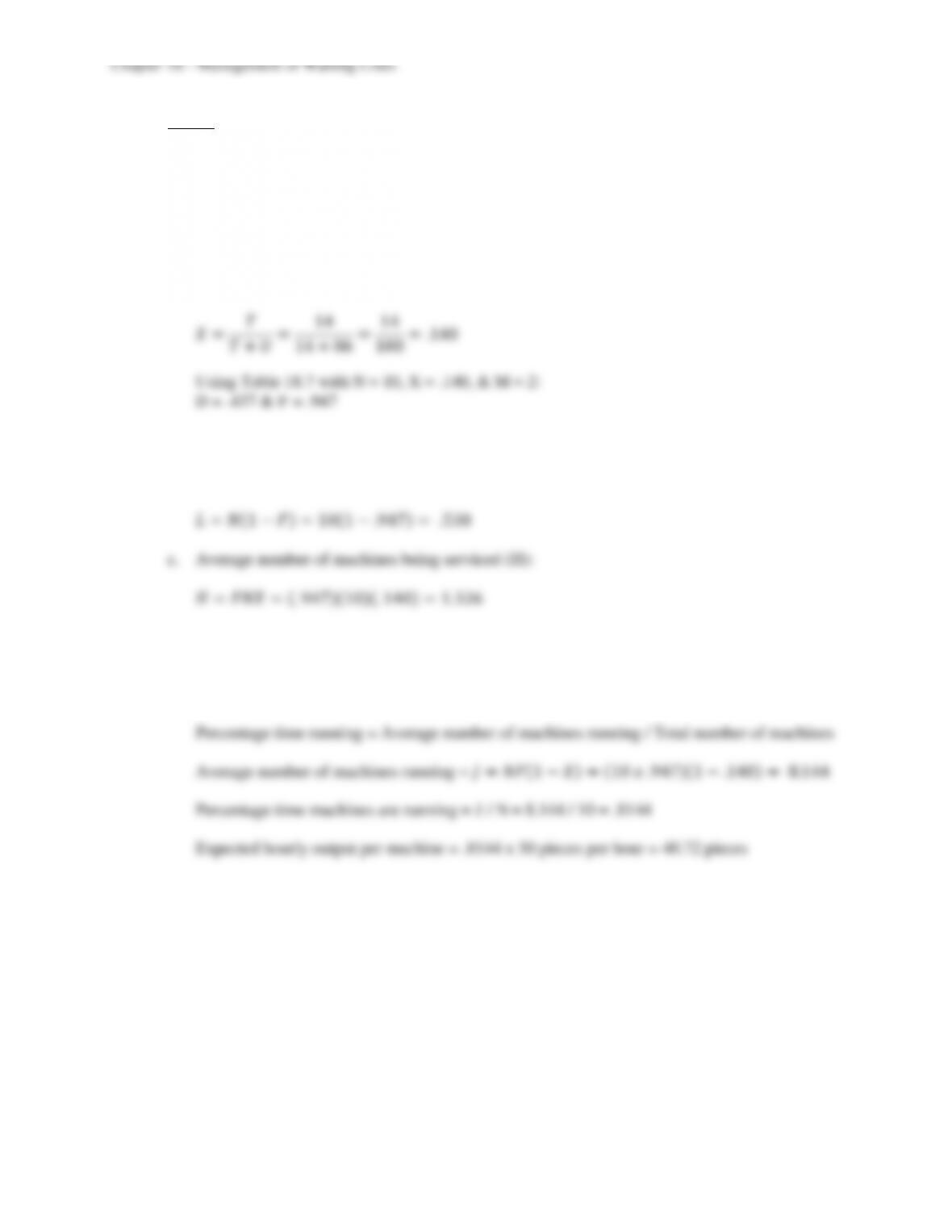
Average number of machines running =
Average number down = N – J
Operator cost = Number of operators x Operator cost per hour
M = 1:
Using Table 18.7 with N = 10, X = .140, & M = 1:
F = .680
M = 2:
Using Table 18.7 with N = 10, X = .140, & M = 2:
F = .947
Average number down = N – J = 10 – 8.144 = 1.856
Machine downtime cost per hour = 1.856 x $70 = $129.92
M = 3:
Using Table 18.7 with N = 10, X = .140, & M = 3:
F = .991
Average number down = N – J = 10 – 8.523 = 1.477
Chapter 18 – Management of Waiting Lines
18–20
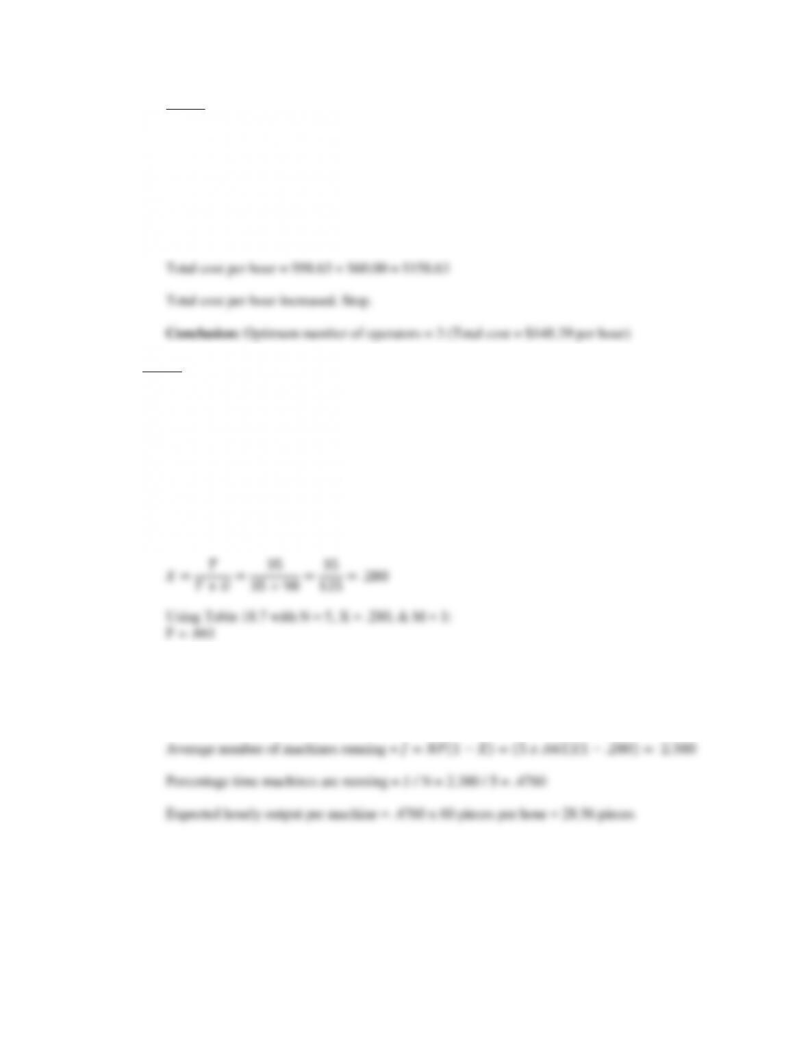
M = 4:
Using Table 18.7 with N = 10, X = .140, & M = 4:
F = .999
Average number down = N – J = 10 – 8.591 = 1.409
Machine downtime cost per hour = 1.409 x $70 = $98.63
Operator cost per hour = 4 x $15.00 = $60.00
11. Given:
N = 5 machines
T = 35 minutes
U = 90 minutes
M = 1 operator
Operator receives $20/hour & machine downtime costs $70/hour/machine.
[Finite–source queuing model]
a. If each machine produces 60 pieces per hour while running, find the average hourly output of
each machine:
Expected hourly output per machine = Percentage time machine is running x Output while
running
Percentage time running = Average number of machines running / Total number of machines