Unlock document.
This document is partially blurred.
Unlock all pages and 1 million more documents.
Get Access
Chapter 18 - Management of Waiting Lines
18-1
Education.
CHAPTER 18
MANAGEMENT OF WAITING LINES
Teaching Notes
Some of the math and calculations can be left out to focus more clearly on the concepts of waiting lines.
For example, all infinite source problems, including single channel (except constant service time) can be
handled using the infinite source queuing table. In the past, queuing presented students with a good bit of
computational requirements, and because of that, students frequently lost sight of the underlying concepts.
With less emphasis on calculations, students can handle individual problems more quickly, allowing an
instructor to assign a greater number of homework problems, and thereby enabling students to enrich their
experience with queuing through a variety of (short) problems.
If you want to shorten the material somewhat, I would suggest omitting the finite source model and/or the
multiple priority model. You can shorten the chapter even more by not assigning problems that require
cost comparisons, although I personally feel that cost comparisons are perhaps the ultimate goal in an
operations management course.
Answers to Discussion and Review Questions
1. Queuing analysis is appropriate in analyzing capacity when the service rate and/or the arrival rate
are highly variable.
2. Variations in the service rate and/or the arrival rate create instances in which demand temporarily
exceeds capacity.
3. Commonly used measures of system performance include the average number of customers
4. The effective system capacity would increase. Consequently, the system could tolerate a higher
arrival rate without experiencing a disproportionate increase in waiting time.
5. Supermarkets advertise specials early in the week to attract customers on slower days and to
6. An infinite source model applies when system entry is unrestricted, or when the potential number
7. The multiple priority approach is appropriate whenever arriving customers are assigned to one of
8. The primary reasons to have customers wait in a single line in a multiple-channel system are to
9. As the utilization increases, the expected length of the waiting line increases. At some point,
slight increases in utilization will have a dramatic increase on the number waiting. This is
Chapter 18 - Management of Waiting Lines
18-2
Taking Stock
1. In waiting line decisions, the primary trade-off is the cost of having too many employees (cost of
service or idle time) vs. the cost of not having enough employees (cost of waiting). If the
2. In assessing the cost of a customer waiting for a service involving the general public, the
3. Technology has had a profound impact on analyzing waiting line systems. First of all, through the
use of computers and simulation studies, we are able to analyze the impact of different levels of
staffing on waiting lines very rapidly. Sophisticated computer systems enable us to perform what-
if analysis and rapidly show the simulated results with different arrival rates and service times.
Technology has improved waiting line performance by allowing managers to use computers to
Critical Thinking Exercises
1. Despite management’s best efforts, in some instances it is not feasible to shorten waiting times.
2. a. We know that as utilization increases, waiting times increase exponentially. Conversely,
when utilization decreases (as would be the case when the service rate doubles), we would
expect a disproportionate decrease in the waiting time, i.e., greater than 50%.
b. With an arrival rate of 8 customers per hour and a service rate of 10 customers per hour:
Chapter 18 - Management of Waiting Lines
18-3
Education.
One important implication is that even small increases in the service rate can yield significant
reductions in the average number waiting. For example, increasing the service rate by only a
little more than 14% (from 10/hr. to about 11.43/hr.) would actually cut the average number
waiting in line almost in half (from 3.200 to 1.633 customers).
3. Relevant factors include the travel distance in terms of time and cost for a centralized location vs.
two or more separate locations; the increased staffing and equipment costs to have workers and
4. Mass customization involves providing standardized services or goods, while incorporating some
degree of customization. Mass customization may be applied at the Eat Now restaurant by
streamlining and standardizing the operations such that it becomes more efficient and faster to
serve the customers while trying to maintain as many of the menu options as possible. However,
5. Student answers will vary. Some possible answers are shown below:
If a manager decided to fire workers to decrease staffing costs, and revenues and profits
decreased disproportionately, this action would violate the Utilitarian Principle.
Chapter 18 - Management of Waiting Lines
18-4
Solutions
1. a. Given:
= 3 customers/hour
= 5 customers/hour
M = 1
[Single Server, Exponential Service Time, M/M/1]
)35(5
)(
q
3) Average waiting time (hours) (Wq):
b. Given:
= 3 repair calls/8-hour day
Mean service time = 2 hours (assume Poisson)
M = 1
= 8 / 2 = 4 repair calls/8-hour day
1) Average number of customers waiting in line (Lq):
250.2
)34(4
3
)(
22
q
L
2) System utilization (ρ):
Chapter 18 - Management of Waiting Lines
18-5
Education.
3) Idle time = 1.00 – 0.75 = 0.25 = 25.00%
0.25 x 8 hours/day = 2.00 hours per day idle
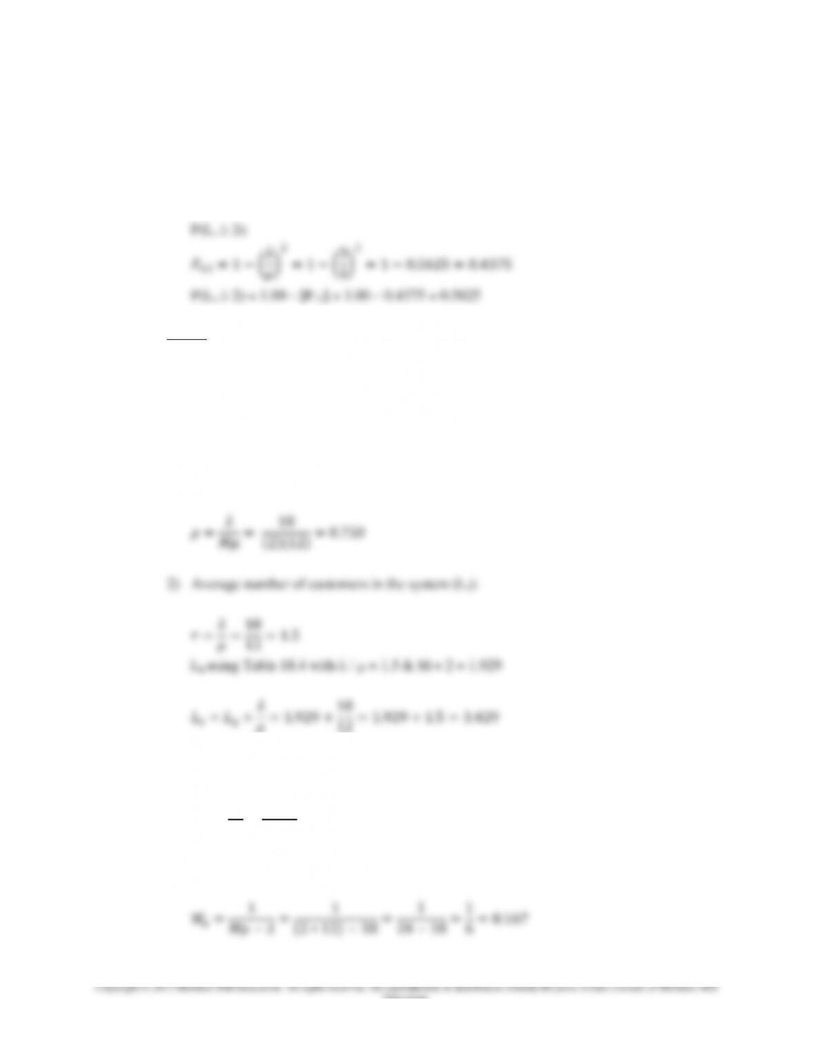
4) Probability of two or more customers in the system:
c. Given:
= 18 customers/hour
= 12 customers/hour
M = 2
[Multiple Servers, M/M/S]
1) System utilization (ρ):
3) Average waiting time for all customers (hours) (Wq):
4) Average waiting time for an arrival not immediately served (hours) (Wa):
18-6
2. Given:
Mean service time = 30 seconds/customer (constant)
= 80 customers/hour
M = 1
[Single Server, Constant Service Time, M/D/1]
Must determine firstμ
= (3600 seconds/hour / 30 seconds/customer) = 120 customers/hour
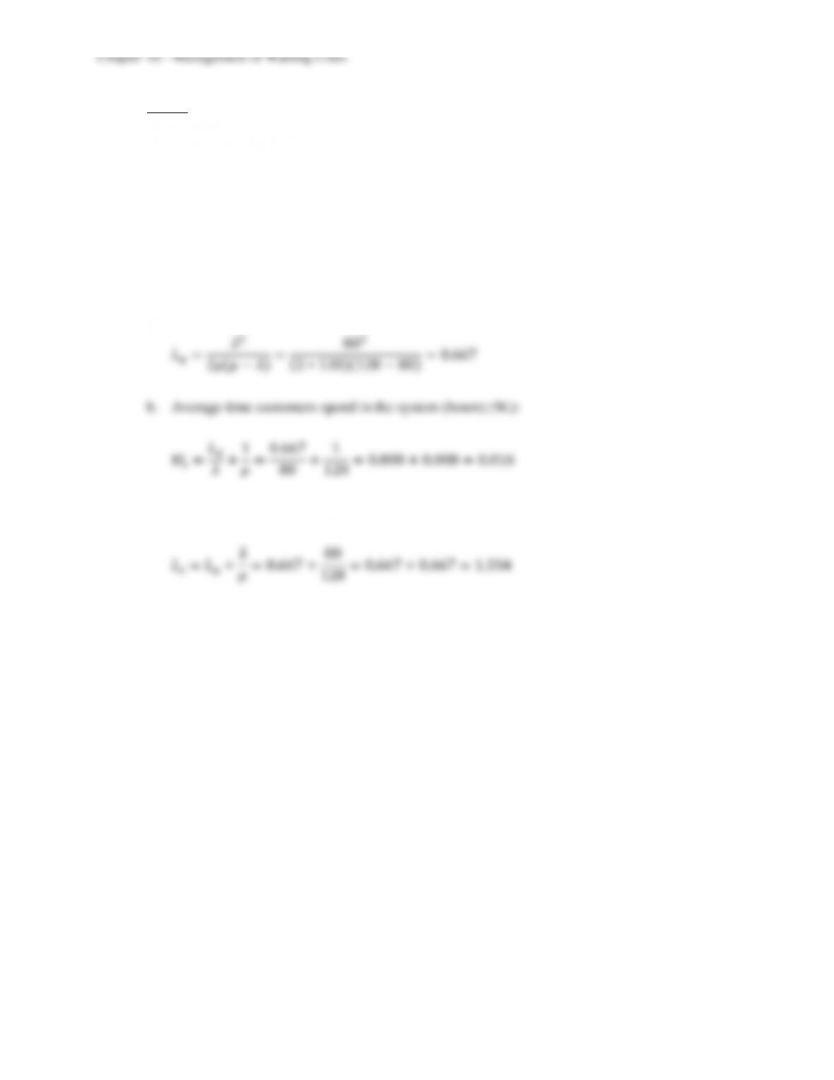
a. Average number of customers waiting in line (Lq):
c. Average number of customers in the system (Ls):
18-7
Education.
3. Given:
Customers arrive at a rate = one every other minute (Poisson)
Mean service time = 90 seconds/customer (exponentially distributed)
M = 1
[Single Server, Exponential Service Time, M/M/1]
We must determine and first (we will use hours)μ
= 1 customer/2 minutes x 60 minutes/hour = 30 customers/hour
= 3600 minutes/hour / λ0 seconds/customer = 40 customers/hour
a. Average time customers spend at the machine, wait time + transaction time (hours) (Ws):
250.2
)3040(40
30
)(
22
q
L
075.0
30
25.2
q
q
L
W
00
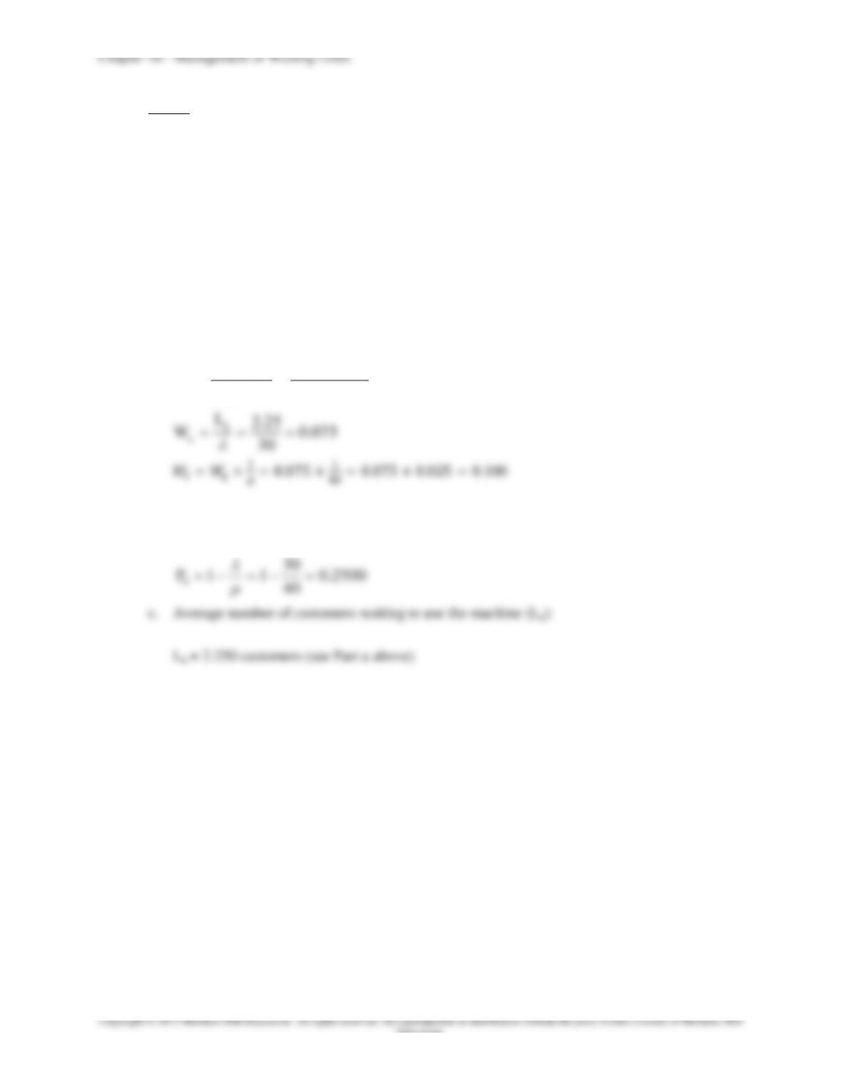
b. Probability that a customer will not have to wait (P0):
2500.0
40
30
11
0
P
c. Average number of customers waiting to use the machine (Lq):
Lq = 2.250 customers (see Part a above)
Chapter 18 - Management of Waiting Lines
18-8
4. Given:
We have the following information pertaining to telephone calls to a motel switchboard:
Period
Incoming Rate
(calls per minute)
Ȝ
Service Rate (calls per
minute per operator)
ȝ
Number of
Operators
Morning
1.8
1.5
2
Afternoon
2.2
1.0
3
Evening
1.4
0.7
3
a. Determine the average time callers have to wait and the probability that a caller will have to
wait during each period:
[Multiple Servers, M/M/S]
Morning:
Chapter 18 - Management of Waiting Lines
18-9
Education.
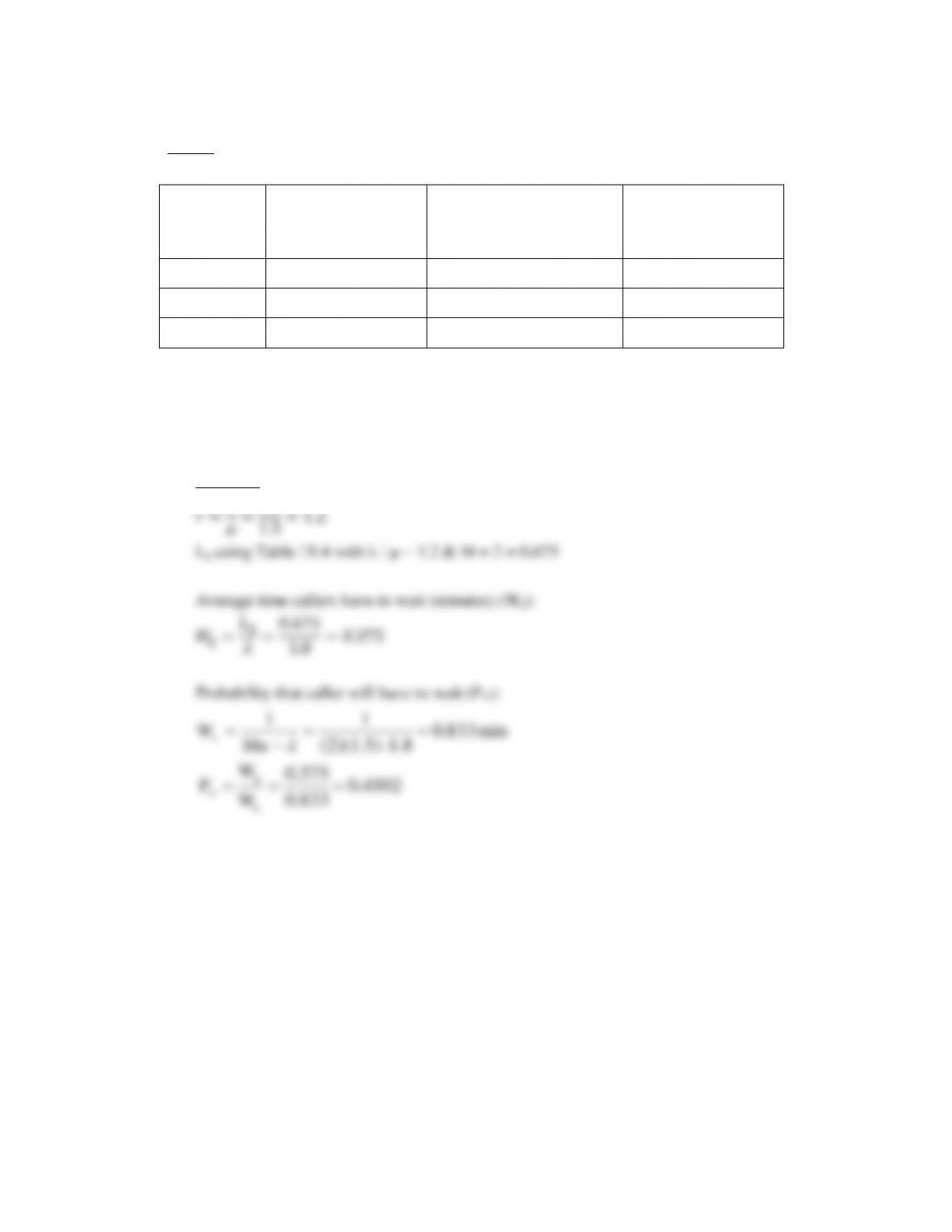
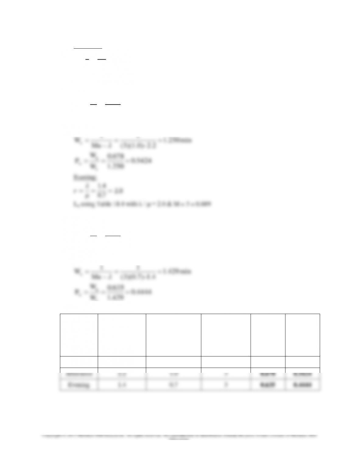
Afternoon:
Lq using Table 18.4 with / = 2.2 & M = 3 = 1.491
Average time callers have to wait (minutes) (Wq):
Probability that caller will have to wait (Pw):
min250.1
2.2- (3)(1.0)
11
Mu
Wa
5424.0
250.1
678.0
a
q
wW
W
P
Evening:
Lq using Table 18.4 with / = 2.0 & M = 3 = 0.889
Average time callers have to wait (minutes) (Wq):
Probability that caller will have to wait (Pw):
min429.1
1.4- (3)(0.7)
11
Mu
Wa
4444.0
429.1
635.0
a
q
wW
W
P
The table below lists the wait time and probability that a caller will have to wait:
Period
Incoming Rate
(calls per
minute)
Ȝ
Service Rate
(calls per minute
per operator)
ȝ
Number of
Operators
Average
Wait
Time
(min.)
Wq
Probably
Caller
Will Have
to Wait
Pw
Morning
1.8
1.5
2
0.375
0.4502
Afternoon
2.2
1.0
3
0.678
0.5424
Evening
1.4
0.7
3
0.635
0.4444
Chapter 18 - Management of Waiting Lines
18-10
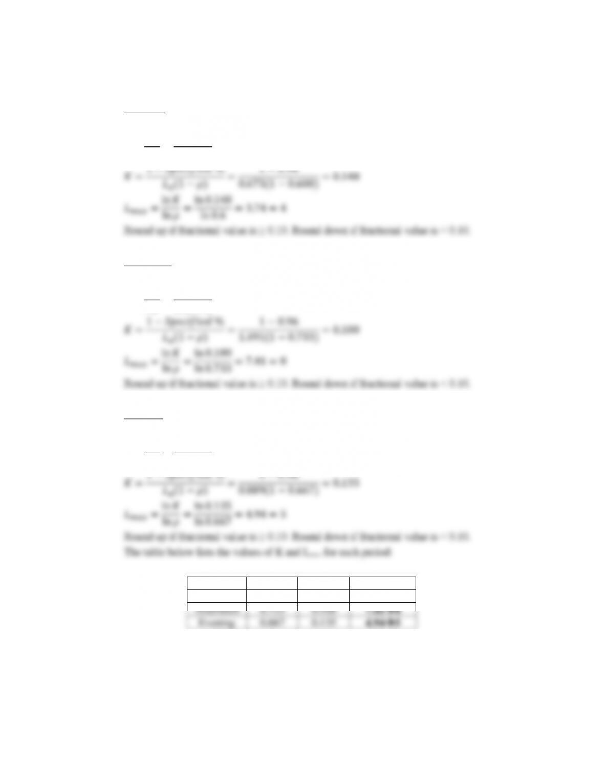
b. For each case above, determine the maximum line length for a probability of 96%:
Morning:
= 1.8, = 1.5, M = 2, Lq = 0.675, r = 1.2
Afternoon:
= 2.2, = 1.0, M = 3, Lq = 1.491, r = 2.2
Evening:
= 1.4, = 0.7, M = 3, Lq = 0.889, r = 2.0
Period
K
Lmax
Morning
0.600
0.148
3.744
Afternoon
0.733
0.100
7.418
Evening
0.667
0.135
4.945


