Chapter 11 – Aggregate Planning and Master Scheduling
11–41
Education.
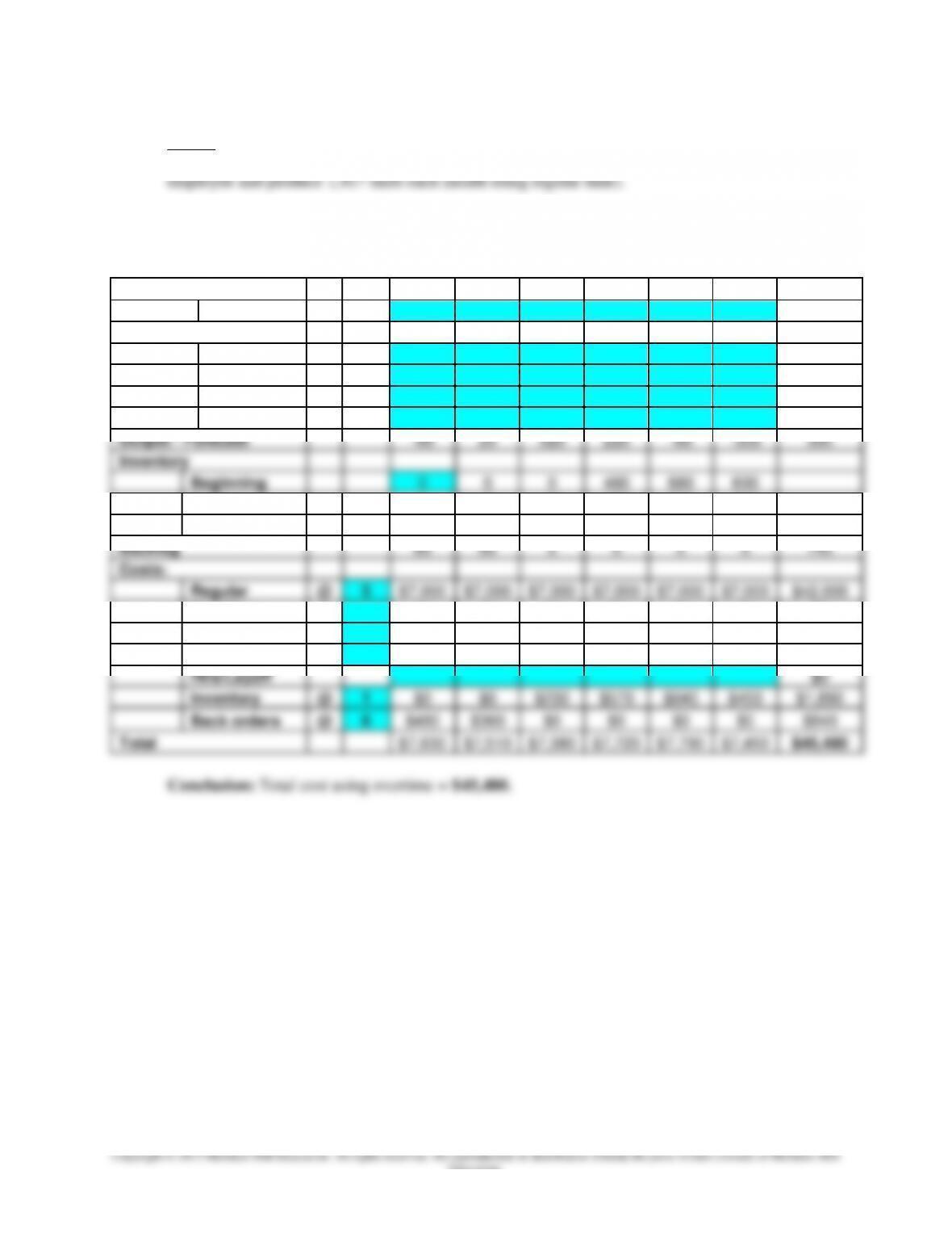
Step 4: Compare the costs of Option 1 (keep the same number of employees, produce 1,400 units
per month using regular time, and produce 100 units total using overtime) vs. Option 2 (hire 1
Option 1: Maintain 28 employees & produce 100 units total using overtime in equal
amounts in Months 1- 5:
Period
1
2
3
4
5
6
Total
Forecast
1,500
1,400
900
1,200
1,500
1,700
8,200
Output
Regular
1,400
1,400
1,400
1,400
1,400
1,400
8,400
Part Time
0
Overtime
20
20
20
20
20
100
Subcontract
0
Output – Forecast
–80
20
520
220
–80
–300
300
Inventory
Beginning
0
0
0
460
680
600
Ending
0
0
460
680
600
300
Average
0
0
230
570
640
450
1,890
Backlog
80
60
0
0
0
0
140
Costs:
Regular
@
5
$7,000
$7,000
$7,000
$7,000
$7,000
$7,000
$42,000
Part Time
@
$0
$0
$0
$0
$0
$0
$0
Overtime
@
7.5
$150
$150
$150
$150
$150
$0
$750
Subcontract
@
$0
$0
$0
$0
$0
$0
$0
Hire/Layoff
$0
Inventory
@
1
$0
$0
$230
$570
$640
$450
$1,890
Back orders
@
6
$480
$360
$0
$0
$0
$0
$840
Total
$7,630
$7,510
$7,380
$7,720
$7,790
$7,450
$45,480
Conclusion: Total cost using overtime = $45,480.
Chapter 11 – Aggregate Planning and Master Scheduling
11–42
Education.
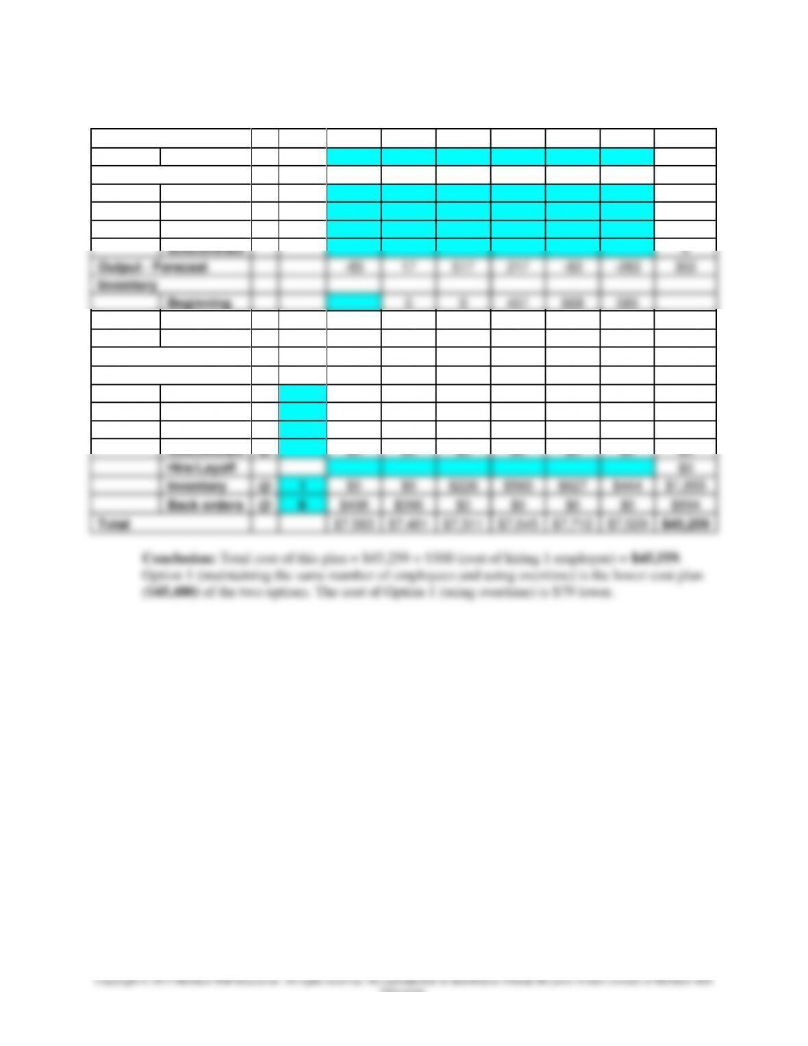
Option 2: Hire 1 worker & produce 1,417 units every month using regular time:
Period
1
2
3
4
5
6
Total
Forecast
1,500
1,400
900
1,200
1,500
1,700
8,200
Output
Regular
1,417
1,417
1,417
1,417
1,417
1,417
8,502
Part Time
0
Overtime
0
Subcontract
0
Output – Forecast
–83
17
517
217
–83
–283
302
Inventory
Beginning
0
0
451
668
585
Ending
0
0
451
668
585
302
Average
0
0
226
560
627
444
1,855
Backlog
83
66
0
0
0
0
149
Costs:
Regular
@
5
$7,085
$7,085
$7,085
$7,085
$7,085
$7,085
$42,510
Part Time
@
$0
$0
$0
$0
$0
$0
$0
Overtime
@
7.50
$0
$0
$0
$0
$0
$0
$0
Subcontract
@
$0
$0
$0
$0
$0
$0
$0
Hire/Layoff
$0
Inventory
@
1
$0
$0
$226
$560
$627
$444
$1,855
Back orders
@
6
$498
$396
$0
$0
$0
$0
$894
Total
$7,583
$7,481
$7,311
$7,645
$7,712
$7,529
$45,259
Chapter 11 – Aggregate Planning and Master Scheduling
11–43
Education.
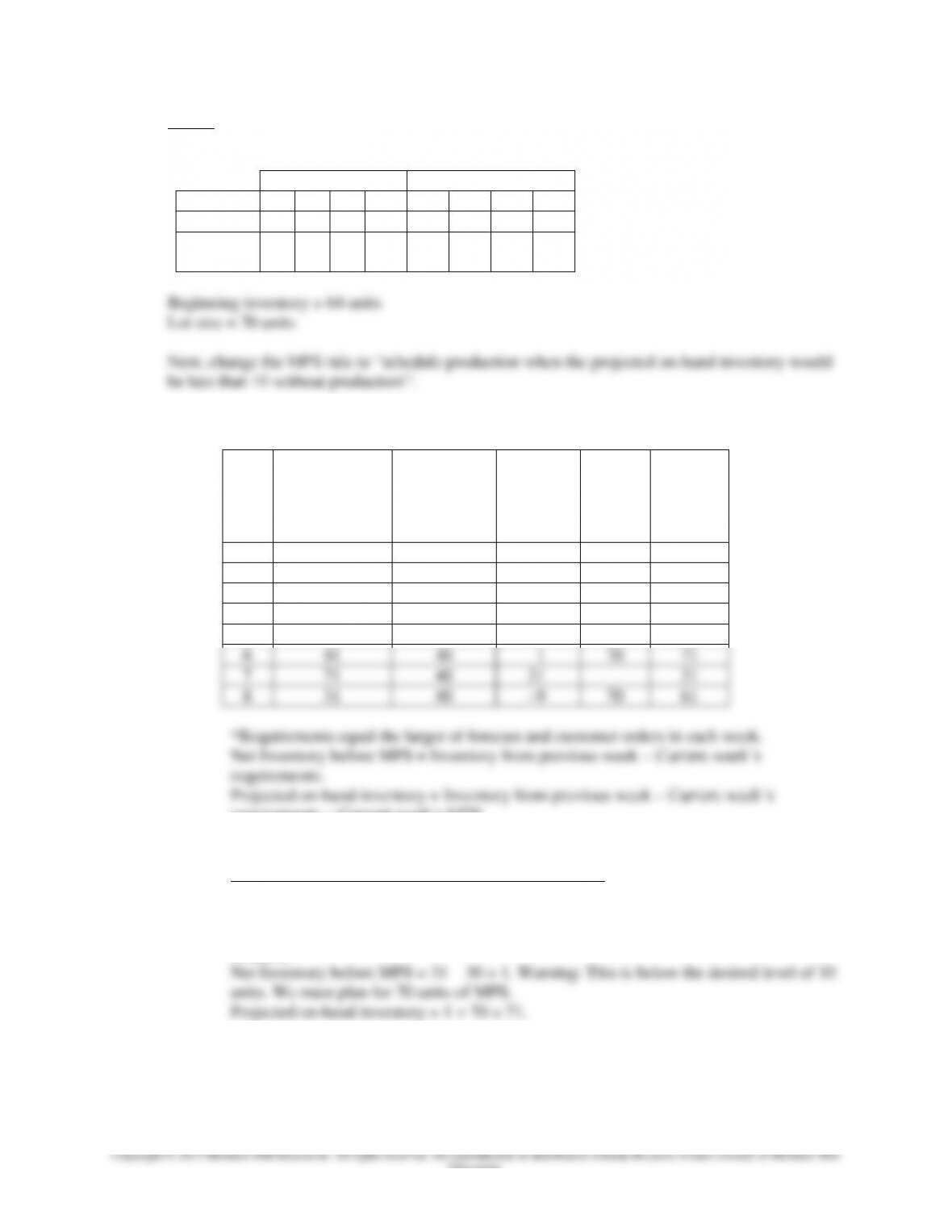
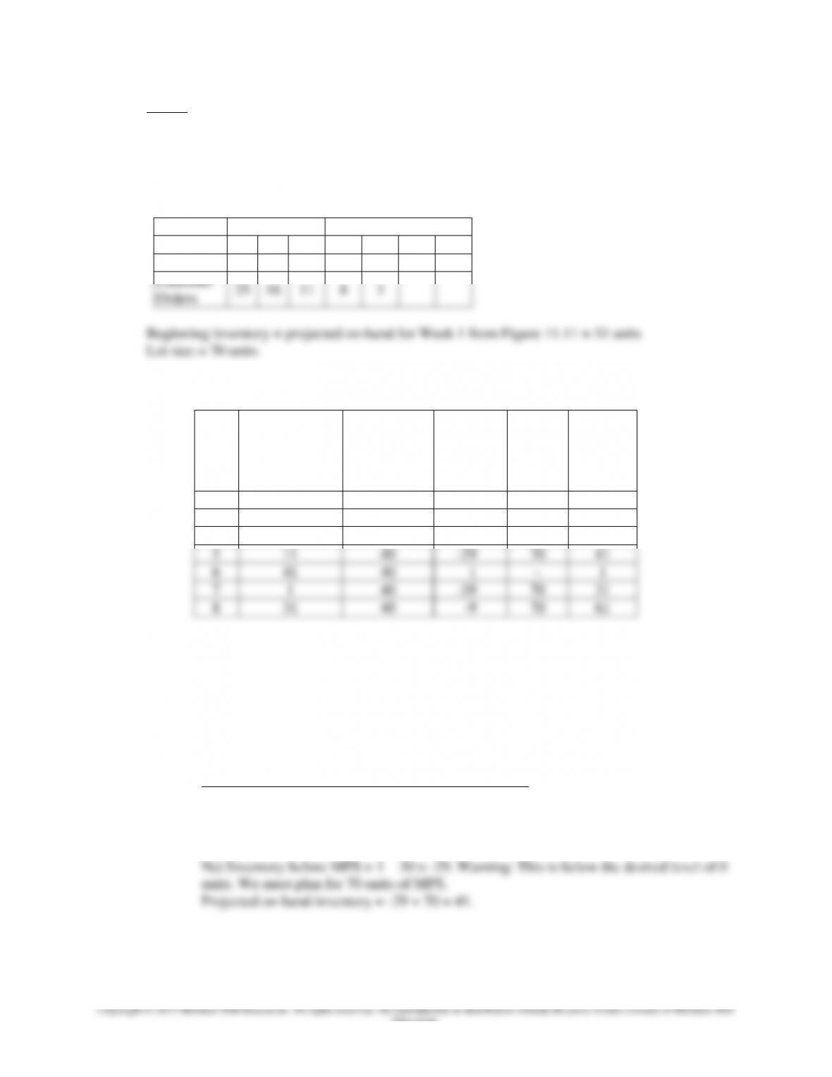
19. Given:
Use the industrial pumps information from Figure 11.11:
June
July
1
2
3
4
5
6
7
8
Forecast
30
30
30
30
40
40
40
40
Customer
Orders
33
20
10
4
2
The calculations for MPS and projected on-hand inventory are shown below:
Week
Inventory From
Previous Week
Requirements*
Net
Inventory
before
MPS
(70)
MPS
Projected
On-hand
Inventory
1
64
33
31
–
31
2
31
30
1
70
71
3
71
30
41
–
41
4
41
30
11
–
11
5
11
40
–29
70
41
6
41
40
1
70
71
7
71
40
31
–
31
8
31
40
–9
70
61
requirements + Current week’s MPS.
Note: We need a MPS quantity whenever Net Inventory before MPS < 10 units.
Example calculations for projected on-hand inventory:
Week 1:
Net Inventory before MPS = 64 – 33 = 31. No MPS is needed.
Projected on-hand inventory = 31 + 0 = 31.
Week 2:
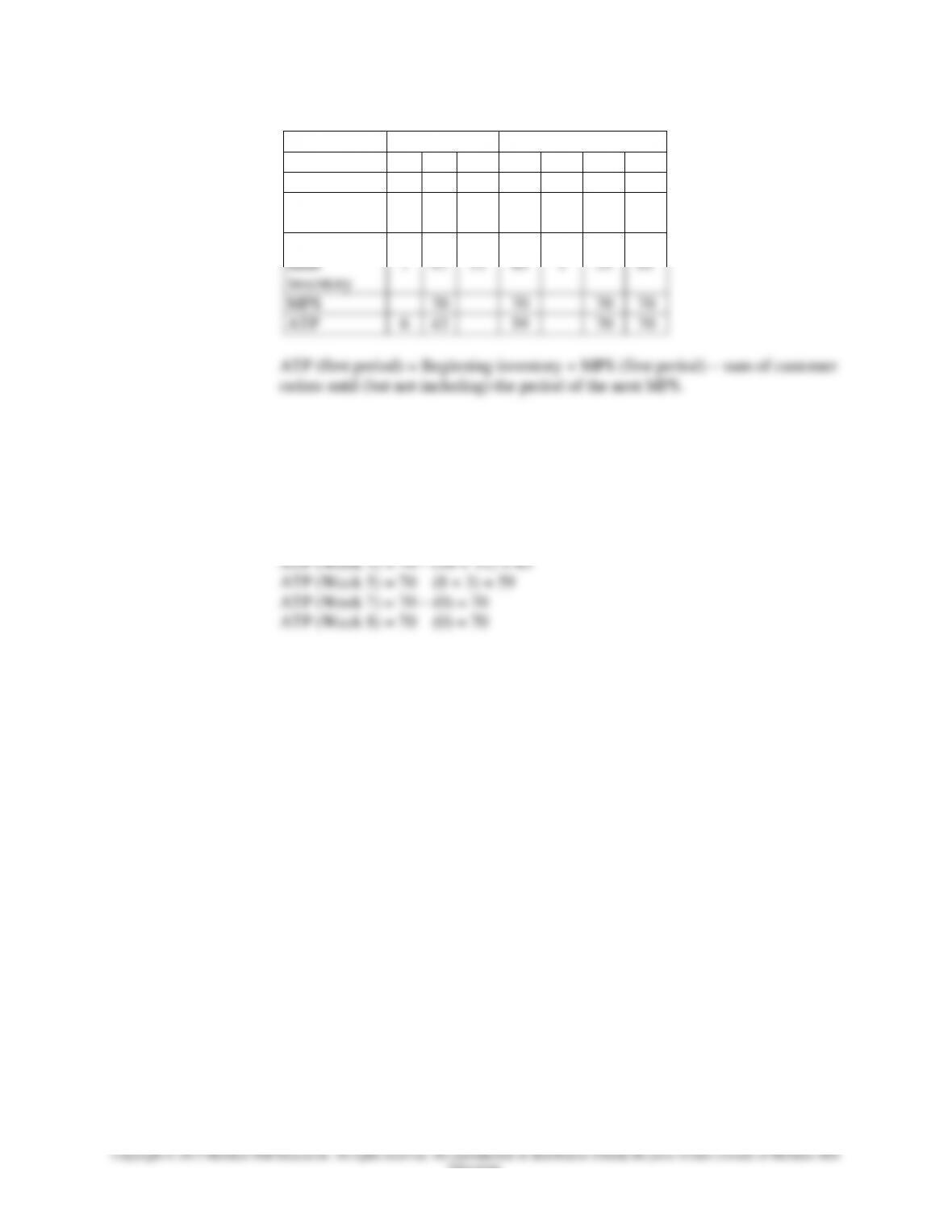
The final MPS is shown below:
Chapter 11 – Aggregate Planning and Master Scheduling
11–44
Education.
Beg. Inv. = 64
June
July
1
2
3
4
5
6
7
8
Forecast
30
30
30
30
40
40
40
40
Customer
Orders
33
20
10
4
2
Projected on-
hand
inventory
31
71
41
11
41
71
31
61
MPS
70
70
70
70
ATP
31
36
68
70
70
ATP (first period) = Beginning inventory + MPS (first period) – sum of customer
orders until (but not including) the period of the next MPS.
ATP (other periods) = MPS (current period) – sum of customer orders until (but
not including) the period of the next MPS.
*We calculate ATP in the first period and in all other periods with MPS
quantities.
ATP (Week 1) = 64 + 0 – (33) = 31
ATP (Week 2) = 70 – (20 + 10 + 4) = 36
Chapter 11 – Aggregate Planning and Master Scheduling
11–45
Education.
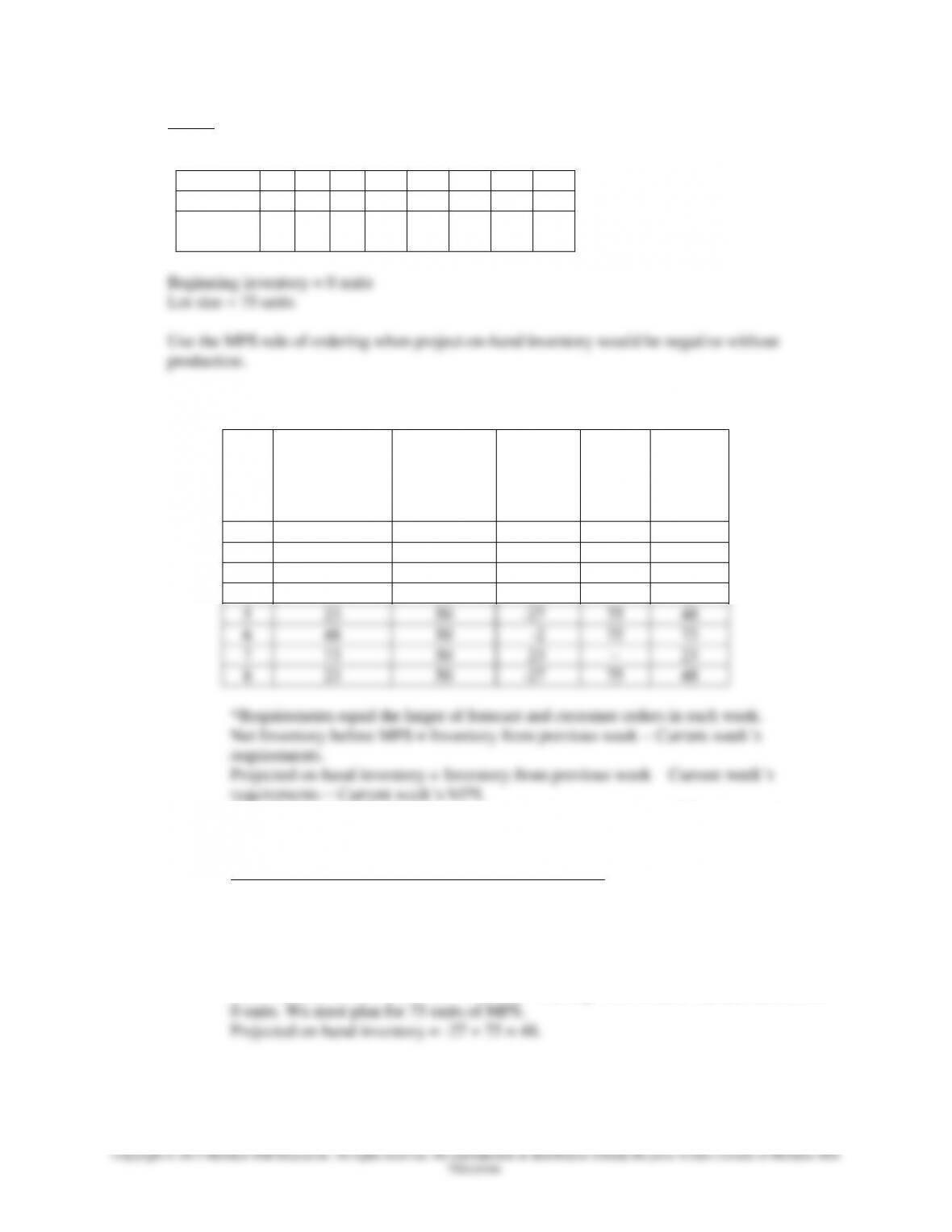
20. Given:
Update the information from Figure 11.11:
It is now the end of Week 1. Customer orders are 25 for Week 2, 16 for Week 3, 11 for Week 4, 8
for Week 5, and 3 for Week 6. Use the MPS rule of ordering when project on-hand inventory
would be negative without production.
June
July
2
3
4
5
6
7
8
Forecast
30
30
30
40
40
40
40
Customer
Orders
25
16
11
8
3
Beginning inventory = projected on-hand for Week 1 from Figure 11.11 = 31 units
Lot size = 70 units
The calculations for MPS and projected on-hand inventory are shown below:
Week
Inventory From
Previous Week
Requirements*
Net
Inventory
before
MPS
(70)
MPS
Projected
On-hand
Inventory
2
31
30
1
–
1
3
1
30
-29
70
41
4
41
30
11
–
11
5
11
40
-29
70
41
6
41
40
1
–
1
7
1
40
-39
70
31
8
31
40
-9
70
61
*Requirements equal the larger of forecast and customer orders in each week.
Net Inventory before MPS = Inventory from previous week – Current week’s
requirements.
Projected on-hand inventory = Inventory from previous week – Current week’s
requirements + Current week’s MPS.
Note: We need a MPS quantity whenever Net Inventory before MPS < 0 units (i.e.,
when it is negative).
Example calculations for projected on-hand inventory:
Week 2:
Net Inventory before MPS = 31 – 30 = 1. No MPS is needed.
Projected on-hand inventory = 1 + 0 = 1.
Week 3:
The final MPS for Weeks 2 – 8 is shown below:
Chapter 11 – Aggregate Planning and Master Scheduling
11–46
Education.
June
July
Beg. Inv. = 31
2
3
4
5
6
7
8
Forecast
30
30
30
40
40
40
40
Customer
Orders
25
16
11
8
3
Projected on-
hand
inventory
1
41
11
41
1
31
61
MPS
70
70
70
70
ATP
6
43
59
70
70
ATP (first period) = Beginning inventory + MPS (first period) – sum of customer
orders until (but not including) the period of the next MPS.
ATP (other periods) = MPS (current period) – sum of customer orders until (but
not including) the period of the next MPS.
*We calculate ATP in the first period and in all other periods with MPS
quantities.
ATP (Week 2) = 31 + 0 – (25) = 6
Chapter 11 – Aggregate Planning and Master Scheduling
11–47
21. Given:
We have the following forecasts and customer orders over the next eight weeks:
1
2
3
4
5
6
7
8
Forecast
50
50
50
50
50
50
50
50
Customer
Orders
52
35
20
12
The calculations for MPS and projected on-hand inventory are shown below:
Week
Inventory From
Previous Week
Requirements*
Net
Inventory
before
MPS
(75)
MPS
Projected
On-hand
Inventory
1
0
52
-52
75
23
2
23
50
-27
75
48
3
48
50
-2
75
73
4
73
50
23
–
23
5
23
50
-27
75
48
6
48
50
-2
75
73
7
73
50
23
–
23
8
23
50
-27
75
48
*Requirements equal the larger of forecast and customer orders in each week.
Net Inventory before MPS = Inventory from previous week – Current week’s
requirements.
Projected on-hand inventory = Inventory from previous week – Current week’s
requirements + Current week’s MPS.
Note: We need a MPS quantity whenever Net Inventory before MPS < 0 units (i.e.,
when it would be negative).
Example calculations for projected on-hand inventory:
Week 1:
Net Inventory before MPS = 0 – 52 = –52. Warning: This is below the desired level of 0
units. We must plan for 75 units of MPS.
Projected on-hand inventory = –52 + 75 = 23.
Week 2:
Net Inventory before MPS = 23 – 50 = –27. Warning: This is below the desired level of
The final MPS is shown below: