Chapter 10 – Quality Control
10–21
Education.
Median Test:
Sample 39 was tied with the median. As shown below, the expected number of runs = 20.5.
The expected number of runs will be greater than the observed number or runs (either 18 or
19 depending on how we label Sample 39). If we label Sample 39 as [B], this will increase
the difference between the observed number of runs and the expected number of runs.
Therefore, Sample 39 was labeled as [B] to maximize the ztest statistic.
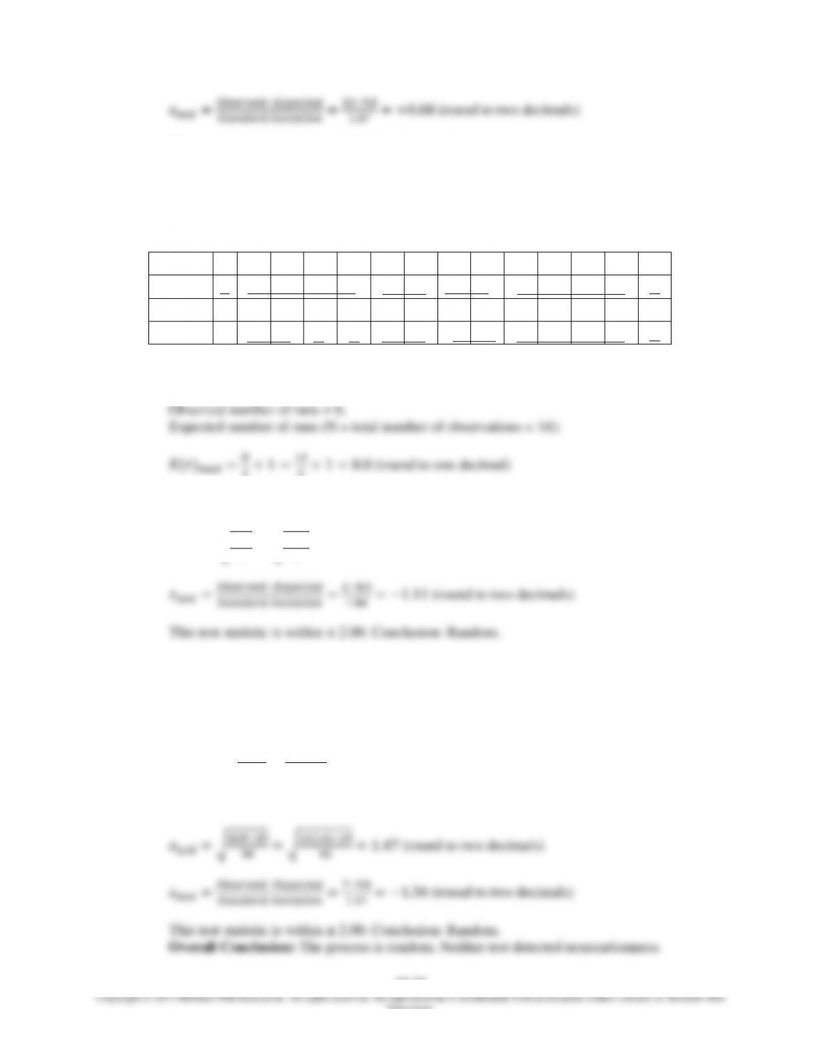
Observed number of runs = 18.
Expected number of runs (N = total number of observations = 39):
This test statistic is within ± 2. Conclusion: Random.
Up/Down Test:
Observed number of runs = 29.
Expected number of runs (N = total number of observations = 39):
(round to one decimal)
Standard deviation:
Overall Conclusion: The process is random. Neither test detected nonrandomness.
Chapter 10 – Quality Control
10–22
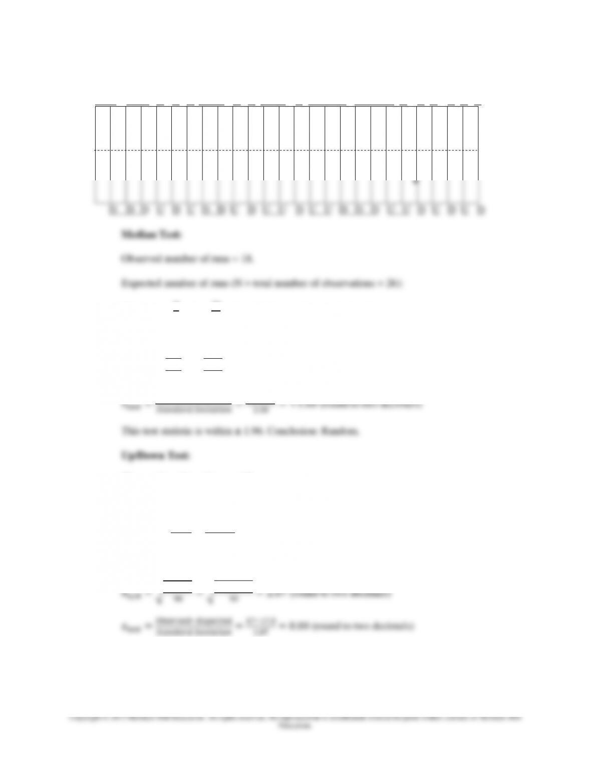
13. a. First control chart is marked with A/B and U/D:
A A B B A B A B B A B A A B A A A B B B A B A B A B
D D D U D U D D U D U U D U U D D D U U D U D U D
(round to one decimal)
Standard deviation:
(round to two decimals)
Expected number of runs (N = number of observations = 26):
(round to one decimal)
Standard deviation:
This test statistic is within ± 1.96. Conclusion: Random.
Overall Conclusion: The process is random. Neither test detected nonrandomness.
Chapter 10 – Quality Control
10–23
Education.
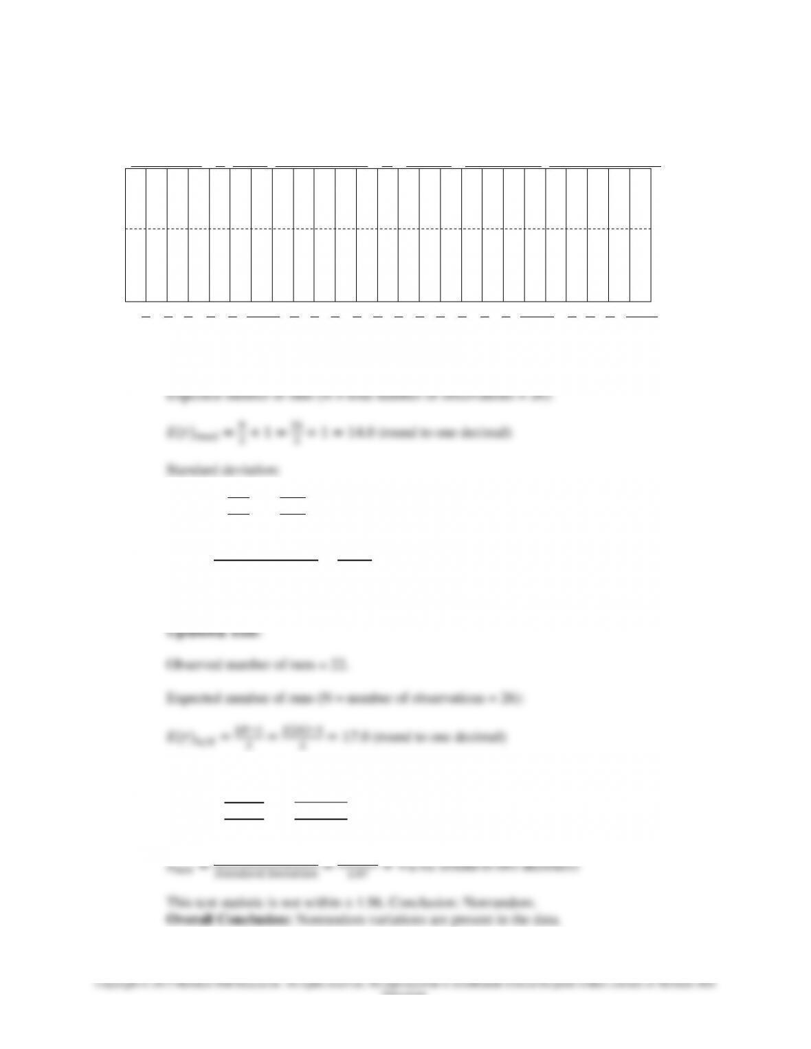
b. Second control chart is marked with A/B and U/D:
A A A A B A A B B B B B A B B B A A A A B B B B B B
U D U D U D D U D U D U D U D U D U D D U D U D D
Median Test:
Observed number of runs = 8.
(round to two decimals)
(round to two decimals)
This test statistic is not within ± 1.96. Conclusion: Nonrandom.
Standard deviation:
(round to two decimals)
Chapter 10 – Quality Control
10–24
14. a. Given:
Test
z-score
Median
+1.37
Up/Down
+1.05
Because neither z-score exceeds +2.00, the process output is probably random.
(round to one decimal)
Standard deviation:
(round to two decimals)
Observed number of runs = 8.
Expected number of runs (round to 1 decimal) (N = number of observations = 20):
(round to one decimal)
(round to two decimals)
This test statistic is not within ± 2.00. Conclusion: Nonrandom.
Overall Conclusion: Nonrandom variations are present in the data.
Chapter 10 – Quality Control
10–25
Education.
c. Given:
Data from Chapter 10, Problem 8:
Cable
1
2
3
4
5
6
7
8
9
10
11
12
13
14
Defects
2
3
1
0
1
3
2
0
2
1
3
1
2
0
5.1
14
21
c
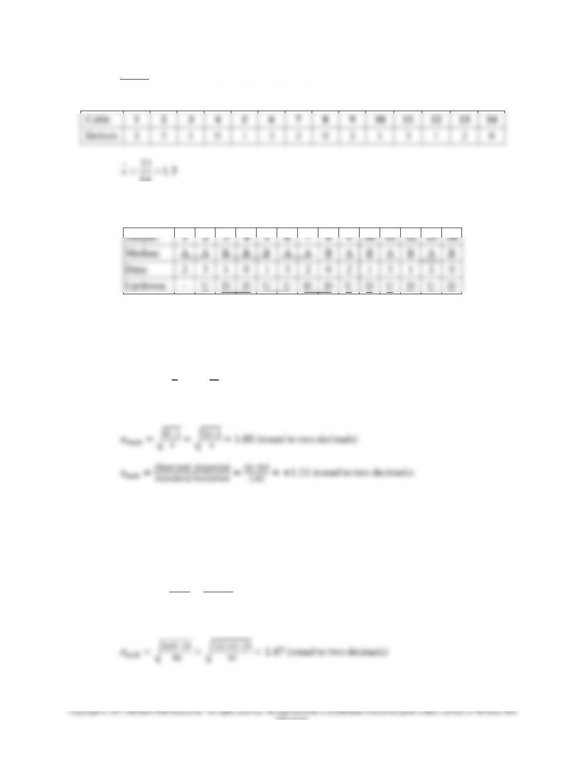
Median is 1.5: A = Above, B = Below, U = Up, D = Down.
Sample:
1
2
3
4
5
6
7
8
9
10
11
12
13
14
Median:
A
A
B
B
B
A
A
B
A
B
A
B
A
B
Data:
2
3
1
0
1
3
2
0
2
1
3
1
2
0
Up/down:
–
U
D
D
U
U
D
D
U
D
U
D
U
D
Median Test:
Observed number of runs = 10.
Expected number of runs (N = total number of observations = 14):
(round to one decimal)
Standard deviation:
This test statistic is within ± 2.00. Conclusion: Random.
Up/Down Test:
Observed number of runs = 10
Expected number of runs (N = total number of observations = 14):
(round to one decimal)
Standard deviation:
Chapter 10 – Quality Control
10–26
Education.
This test statistic is within ± 2.00. Conclusion: Random.
Overall Conclusion: The process is random. Neither test detected nonrandomness.
d. Data from Chapter 10, Problem 7:
Median is 7.5.
Day:
1
2
3
4
5
6
7
8
9
10
11
12
13
14
Median:
B
A
A
A
A
B
B
A
A
B
B
B
B
A
Data:
4
10
14
8
9
6
5
12
13
7
6
4
2
10
Up/down
–
U
U
D
U
D
D
U
U
D
D
D
D
U
Median Test:
Observed number of runs = 6.
(round to one decimal)
Standard deviation:
(round to two decimals)
Up/Down Test:
Observed number of runs = 7
Expected number of runs (N = total number of observations = 14):
(round to one decimal)
Standard deviation:
10–27
Education.
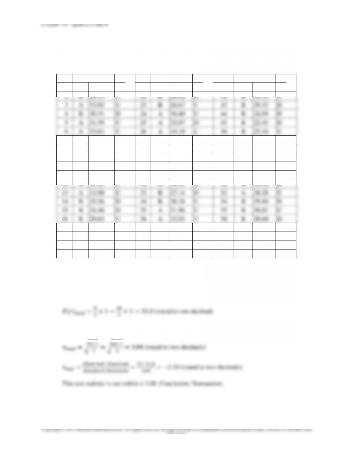
15. Given:
Expense voucher values are provided below. The data already have been converted to A/B and
U/D. Assume a median of 31.
Day
Amount
Day
Amount
Day
Amount
1
B
27.69
21
B
28.60
U
41
B
26.76
D
2
B
28.13
U
22
B
20.02
D
42
B
30.51
U
3
A
33.02
U
23
B
26.67
U
43
B
29.35
D
4
B
30.31
D
24
A
36.40
U
44
B
24.09
D
5
A
31.59
U
25
A
32.07
D
45
B
22.45
D
6
A
33.64
U
26
A
44.10
U
46
B
25.16
U
7
A
34.73
U
27
A
41.44
D
47
B
26.11
U
8
A
35.09
U
28
B
29.62
D
48
B
29.84
U
9
A
33.39
D
29
B
30.12
U
49
A
31.75
U
10
A
32.51
D
30
B
26.39
D
50
B
29.14
D
11
B
27.98
D
31
A
40.54
U
51
A
37.78
U
12
A
31.25
U
32
A
36.31
D
52
A
34.16
D
13
A
33.98
U
33
B
27.14
D
53
A
38.28
U
14
B
25.56
D
34
B
30.38
U
54
B
29.49
D
15
B
24.46
D
35
A
31.96
U
55
B
30.81
U
16
B
29.65
U
36
A
32.03
U
56
B
30.60
D
17
A
31.08
U
37
A
34.40
U
57
A
34.46
U
18
A
33.03
U
38
B
25.67
D
58
A
35.10
U
19
B
29.10
D
39
A
35.80
U
59
A
31.76
D
20
B
25.19
D
40
A
32.23
D
60
A
34.90
U
Median Test:
Observed number of runs = 22
Expected number of runs (N = total number of observations = 60):
Standard deviation:
Chapter 10 – Quality Control
Up/Down Test:
Observed number of runs = 35
Expected number of runs (N = total number of observations = 60):
(round to one decimal)
Standard deviation:
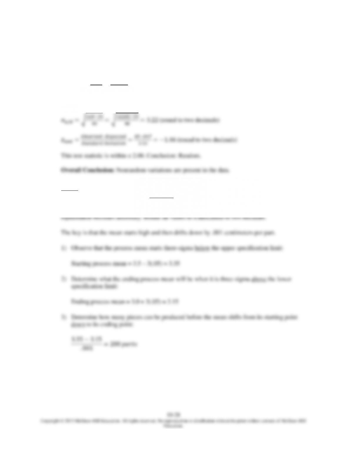
16. Given:
Inside diameter of successive parts decreases at an average rate of .001 centimeters per part.
The process sigma = .05 centimeters. Specifications are set at 3.0 to 3.5 centimeters. A three-
sigma cushion is set. Determine the number of parts that can be processed before tool
10–30
Education.
With a scrap rate of 3% (.03) at Step 3, the output of Step 3 = (1-.03)(.97)(.95x) =
(.97)(.97)(.95x).
Multiplying out: The output of Step 3 = .8939x (round to four decimals).
Let .8939x = 450
19. Given:
Refer back to the data in Example 5. Two additional observations have been taken: the first had
three defects and the second had four defects. Combine these last two with the first eighteen
observations. The original data are shown in the table below. The data already have been
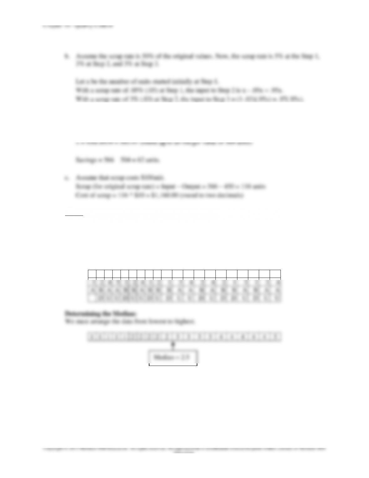
converted to A/B and U/D.
Sample
1
2
3
4
5
6
7
8
9
10
11
12
13
14
15
16
17
18
19
20
3
2
4
5
1
2
4
1
2
1
3
4
2
4
2
1
3
1
3
4
A
B
A
A
B
B
A
B
B
B
A
A
B
A
B
B
A
B
A
A
D
U
U
D
U
U
D
U
D
U
U
D
U
D
D
U
D
U
U
Determining the Median:
We must arrange the data from lowest to highest.
1
1
1
1
1
2
2
2
2
2
3
3
3
3
4
4
4
4
4
5
Median = 2.5