
Chapter 02 – Determination of Interest Rates 6th Edition
1. Determinants of Interest Rates For Individual Securities
a. Inflation
b. Real Riskless Interest Rates & Fisher Effect
Inflation is the rate of change in the overall price level. The Consumer Price Index
(CPI) is the most commonly quoted measure of inflation. The CPI purports to measure
the price level of a market basket of goods and services purchased by the typical urban
consumer.
The Fisher effect states that nominal riskless rates equal real riskless rates plus a
premium for expected inflation. This relationship is the basis for the term structure.
Differences in annual expected inflation rates cause differences in bond rates with
different maturities.
The nominal interest rate is the additional dollars earned from an investment. The real
interest rate is the additional purchasing power earned from an investment. The real
interest rate refers to the marginal gain in units purchased rather than in dollars.
Teaching Tip: Sometimes we think that ex-ante real rates cannot be negative, but they can
because of the convenience yield of liquidity. They have been negative in recent years in
both the U.S. and Japan.
The Fisher Effect relates nominal and real interest rates.
The approximate Fisher effect is given as
i = RIR + Expected (IP)
where i = nominal riskless interest rate, RIR = real riskless interest rate and Expected (IP)
= expected inflation.
The actual Fisher Effect is given as
(1+i) = (1+RIR)*(1+Expected(IP))
The following example illustrates why the actual Fisher Effect is multiplicative:
Suppose “It” originally cost you $1. You have $10 so could buy 10 of “it.”
If inflation is 5%, in one year “it” will cost $1 + .05 =$1.05.
If you invest your $10 and earn 10% + 5% = 15% (the approximate Fisher Effect)
you will get back $10 * 1.15 = $11.50.
Can you buy $10% more of “it?” I.E. can you now buy 10 * 1.1 or 11 of “it?”
11 * $1.05 = $11.55; so you are short 5 cents.
In order to buy 10% more of it you must earn an interest rate equal to (1.10 * 1.05) –
1 = 1.155 – 1 = 15.5% nominal interest.
Then your $10 will grow to $10 * 1.155 = $11.55 and you CAN buy 10% more of it!
Since both P & Q are rising, the rate charged must reflect the increments to both P
and Q.
The difference matters little if inflation is low and/or the time period under
consideration is not very long. In international investing environments where
inflation is much higher than the U.S. is currently experiencing, the difference can
be material.
As of this writing, core inflation measures remain subdued but commodity and food
2-1
Chapter 02 – Determination of Interest Rates 6th Edition
prices are increasing. Even though measured inflation, particularly core inflation which
excludes food and energy, remains low, prices of high frequency purchases such as food
and gas are increasing at a higher rate. Thus, there seems to be more inflation than the
CPI numbers indicate. Moreover, the practice of ‘hedonics’ in inflation calculations adds
some uncertainty about the validity of actual inflation numbers.1 Rising oil prices may
also reduce economic growth. Sustained high oil prices drive up the cost of production
and act as a tax on consumers. Economists estimate that if oil hits $120 a barrel,
economic growth will be substantially reduced.
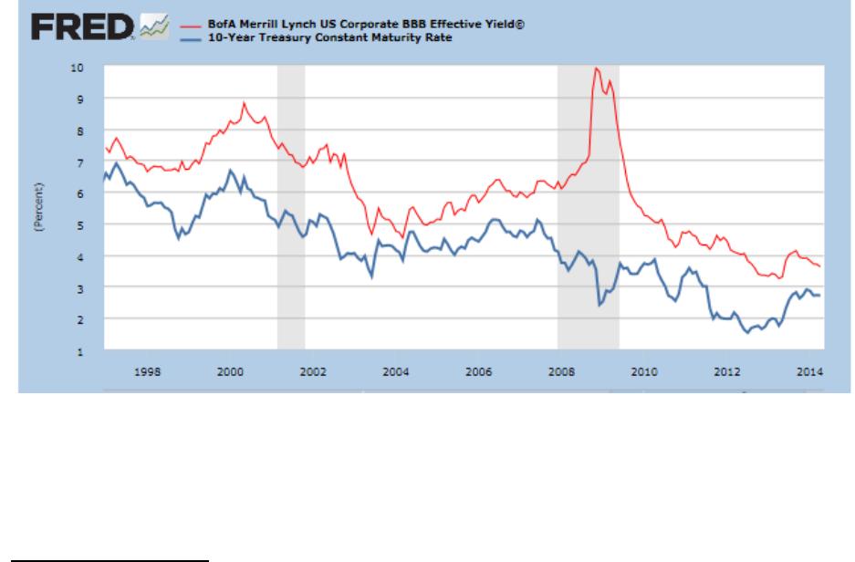
c. Default or Credit Risk
Default risk premiums (DRPs) are increases in required yield needed to offset the
possibility the borrower will not repay the promised interest and principle in full or as
scheduled. According to the Wall Street Journal Online, credit risk premiums on Aa rated
corporate debt relative to Treasuries between March 2010 and March 2011 ranged
between 86.6 and 150 basis points and on Baa rated debt ranged between 172 and 237
basis points. DRPs on high yield debt ranged between 453 and 728 basis points over
Treasuries. DRPs are cyclical, and rise in periods of weak economic conditions such as
the U.S. has been experiencing in recent years. The FRED graph below contains the
yields on the Bank of America Merrill Lynch US Corporate BBB Effective Yield and the
10 year Treasury Constant Maturity Rate. Notice the large increase in the spread during
the recent recession.
1 Hedonics is the ‘art’ of adjusting prices for quality differences over time. For instance, a TV purchased
today that costs the same as a TV purchased several years ago has more features. The price of the new TV
is adjusted downward to reflect the additional technology.
2-2
Chapter 02 – Determination of Interest Rates 6th Edition
d. Liquidity Risk
Liquidity risk premiums are increases in required or promised yields designed to offset
the risk of not being able to sell the asset in timely fashion at fair value. These are similar
to, but not the same as, the liquidity premiums in the term structure discussion. Liquidity
risk can be more significant for some debt instruments than for stocks as many bonds
trade in thin markets.
e. Special Provisions of Covenants
Municipal bond (Muni) rates are lower than similar corporate bonds because interest
(but not capital gains) is exempt from federal taxation. In most states the holder of a
muni bond issued in that state is also exempt from state taxes.
Teaching Tip: Ask students why munis are granted special tax status. What do they
think about industrial development bonds which allow private corporations to issue
tax advantaged munis for certain projects? Note that usage of IDBs has been
restricted in recent years due to over usage by private firms seeking to exploit the tax
advantage of municipals.
Teaching Tip: The municipal bond market is going through a crisis in the spring of
2011 because of concerns with large state budget deficits. Longer term muni bond
rates were between 3.52% and 4.7% in May 2014. It seems unlikely that failures will
occur because the bonds usually carry high priority in state budgets. It seems more
likely that bond payments will crowd out other types of state spending.
Callable bonds have higher required yields than straight bonds because the issuer will
normally call them when rates have dropped, forcing the bondholders to reinvest at
lower interest rates. Although it varies with interest rate expectations the premium on
a callable bond might be 30 to 50 basis points.
Convertible bonds have lower yields than straight bonds because the bondholder has
the right to convert them to preferred or common stock at their choice. Offering a
conversion feature may save 100 to 200 basis points, ceteris paribus. In most cases
however, the stock has to appreciate 15%-25% over the at issue price in order to make
conversion attractive.
f. Term to Maturity
The term structure depicts the relationship between maturity and yields for bonds
identical in all respects except maturity. In practice, ‘identical’ means same rating,
liquidity and hopefully the same coupon (or differential tax effects will be present). The
graph of the term structure can take on any shape, but upward sloping is most common
(meaning longer term bonds promise higher nominal yields). The yield curve was
inverted in Nov 2000 and in parts of 2006 and 2007. Note that for Treasuries, ‘on the
run’ (newly issued) securities often carry price premiums over ‘off the run’ (previously
issued) securities.
In the graph below one can see that long term rates are normally above short term rates,
2-3
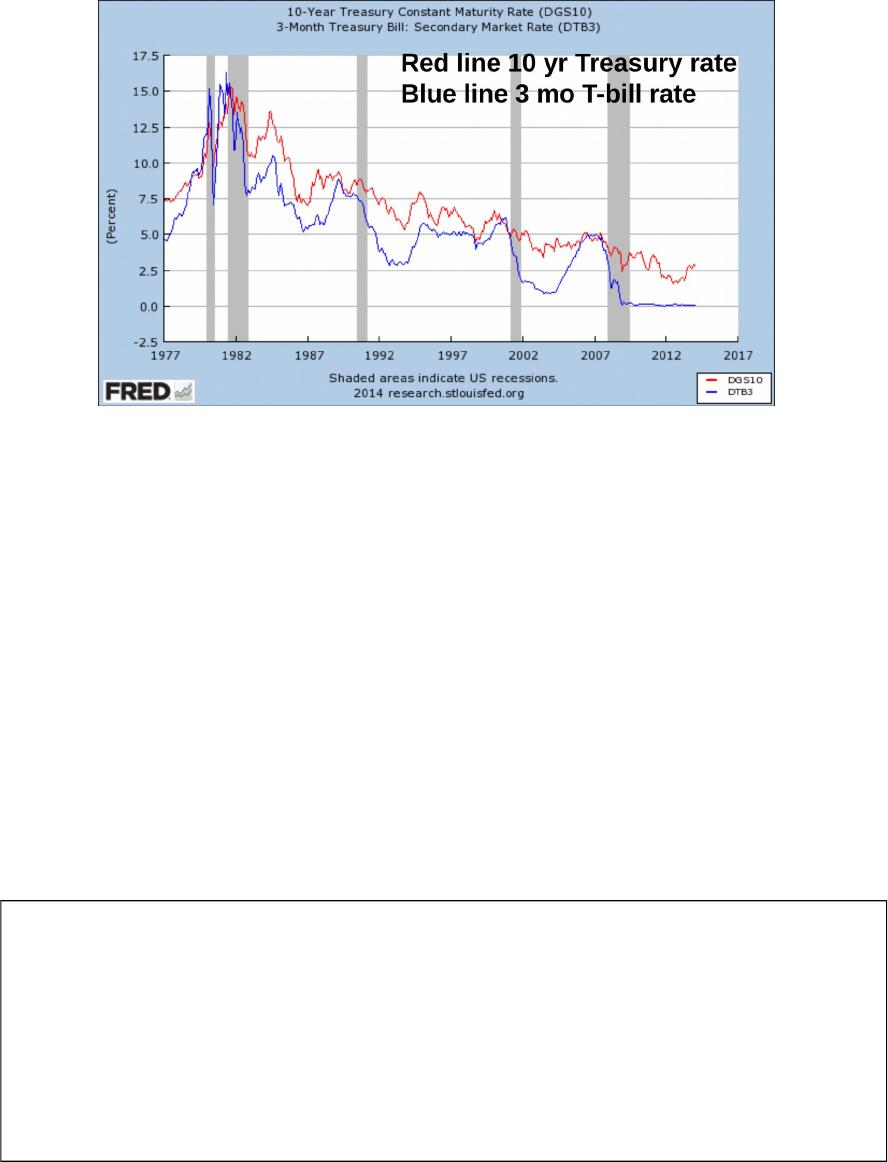
Source: St. Louis Federal Reserve
Chapter 02 – Determination of Interest Rates 6th Edition
although the relationship may change ahead of recessions (depicted by the shaded bars).
g. Summary
ij* = f(Riskless real rate, Expected inflation, Default risk premium, Liquidity risk
premium, Special covenant premium, Maturity risk premium)
The maturity risk premium is explained in Section 5 where it is defined as the premium
for holding a price volatile asset (confusingly called a liquidity premium).
2. Term Structure of Interest Rates
a. Unbiased Expectations Theory (UET)
The UET states that the long term interest rate is the geometric average of the current and
expected future short term rates. A simple arbitrage proof can be used to show this when
interest rates are known with certainty under perfect markets:
If the expected one year rates are 6%, 7% and 8% for the next three years respectively,
and the three year rate is 5%, how could one make money on this relationship?
Using the text’s terminology: 0R1 = 6%, 1R1=7% and 2R1 = 8% but 0R3=5%
The average of the short term one year rates is 7%, but the three year rate is only 5%.
One could borrow any given amount such as $1000 for the full three years and invest that
money one year at a time and rolling over the investment for three years. The borrowing
cost per year is 5% and the average rate of return is 7%. This is a riskless arbitrage under
the given assumptions that would force the three year rate and the average of the one year
2-4

Chapter 02 – Determination of Interest Rates 6th Edition
rates to converge.
The instructor may wish to show this relationship first using simpler arithmetic averages
as above since students often seem to struggle with the concept of geometric averages.
Geometric averages are used to account for compounding; for examples of two or three
years where the rates are similar, the use of arithmetic averages will give almost identical
results if the returns are similar to one another.
For a series of holding period returns (HPRs) the geometric average can be found as:
1)1(
/1
1
N
N
T
T
HPRAverageGeometric
For example if we have a time series of three returns of 10%, -15% and 12% the
arithmetic and geometric averages are 2.33% and 1.55% respectively:
Interpreting the UET
The UET has different possible interpretations.2 It can imply that the return over a given
time horizon should be the same regardless of the bond maturity chosen. For example,
for a 5 year investment horizon the realized rate of return should be the same regardless
of whether a 5 year bond or a 10 year bond is held for 5 years. A second interpretation
may be termed the ‘local expectations’ form of the UET. This version holds that realized
returns will be the same regardless of the bond maturity chosen only for short term
holding periods such as 6 months. The third interpretation is that under the UET an
investor is indifferent between how one arrives at an N year investment by choosing any
bond maturity less than or equal to N and rolling the investment over as needed. For
example, one would be indifferent between investing for N years all at once, or investing
for 1 year and rolling the investment over N-1 times. All three interpretations ignore
interest rate volatility and market imperfections such as transactions costs.
b. Liquidity Premium Theory
If investors prefer shorter maturities to long, they will require a premium to invest for N
years all at once instead of investing for 1 year and rolling the investment over N-1 times.
In other words, the long term rate cannot be the average of the expected short term rates.
The long term rate must equal the average of the short term rates plus what is illogically
called a ‘liquidity premium.’ (It is an illiquidity premium.) The rationale for the shorter
2 This section is drawn from F. Fabozzi, The Handbook of Fixed Income Securities, 8th ed., McGraw-Hill,
2012.
2-5
%33.2
3
%)12%15%10(
AverageArithmetic
%55.1112.185.010.1
3/1
AverageGeometric

Chapter 02 – Determination of Interest Rates 6th Edition
maturity preference is that with uncertainty about future rates, it is riskier to invest long
term rather than investing for a shorter time and rolling the investment over because it is
harder to forecast rates further in the future and longer term investments are more price
volatile. This is a modification of the UET, but it does not invalidate the logic of the UET.
It does imply that long term rates are biased forecasters of expected future short term
rates. We don’t know very much about the size of the liquidity premiums. They increase
with maturity, and probably do not get much over 100 to 200 basis points.3
c. Market Segmentation Theory
The market segmentation theory claims that there are two or three distinct maturity
segments (the segments are ill-defined) and market participants will not venture out of
their preferred segment, even if favorable rates may be found in a different maturity. A
less extreme version posits that a sufficient interest rate premium may induce investors to
switch maturity segments. The idea behind segmentation is that institutions naturally
have liabilities of a distinct maturity, e.g., life insurers have long term liabilities, so they
will not invest short term. Hence, there is no or only a very weak relationship between
interest rates of different maturities and supply and demand of a given maturity sets the
individual interest rates. By inference, there is no reason to construct a term structure as
there is no relationship between long term rates and expected future short term rates.
This is unlikely to strictly hold because it suggests that opportunities to take advantage of
mispricing of securities will not be exploited. For example if the 10 year bond rate is
much higher than warranted by expectations, one could buy the 10 year bond and short a
9 year bond. If the rates on different maturities are far enough out of line with
expectations, some entity will seek to exploit the profit opportunity. If existing investors
will not exploit the opportunity, new investors will emerge to do so in a capitalist system.
In fact this is a typical hedge fund strategy. On the other hand, daily changes in supply
and demand and changes in non-price conditions can certainly cause long term rates to
diverge from the average of expected future short term rates. These create profit
opportunities for astute bond traders. If bond markets are reasonably efficient, these
profit opportunities should not persist long.
3. Forecasting Interest Rates
A forward rate is a rate that can be imputed from the existing term structure. It is a
mathematical tautology that given a set of long term zero coupon spot rates one can find
the set of individual one year forward rates. For instance using the books terminology:
3 Although this is not in the text, the preferred habitat theory posited by Modigliani and Sutch,
Innovations in Interest rate Policy, American Economic Review, May 1966, pp.178-197, suggests it is
possible for liquidity premiums to be negative. If investors have long investment horizons it is actually less
risky for them to hold long duration bonds (as opposed to short duration) to minimize their interest rate
risk. If the majority of investors have long time horizons then it would be riskier to hold short term, low
duration investments. This could make long term investments preferable to short term, implying that the
liquidity premium would have to be negative.
2-6

Chapter 02 – Determination of Interest Rates 6th Edition
(1+1R6)6 = (1+1R5)5 * (1+5F1)
(1+1R5)6 = (1+1R4)4 * (1+4F1) …
where 1R6 and 1R5 are the long term zero coupon spot rates from today to year 6 and 5
respectively and F stands for a forward rate. The first subscript refers to the loan
origination date, but the textbook confusingly uses 1 instead of 0 as is normal to represent
today. The second subscript refers to the term to maturity. Since all the spot rates are
known one can construct the full set of forward rates, iF1, from them.
Teaching Tip: The text implies that the Treasury issues zero coupon bonds across the
maturity structure but this is not true. Most Treasuries beyond one year pay coupons,
although a strip program exists. One can calculate the series of zero coupon spot rates
implied by the Treasury yields via a process called bootstrapping. The zero coupon
rates are called spot rates. Not all spot rates are available because the Treasury does not
issue every possible maturity. Newly issued securities are preferred because they are
more liquid. The missing spot rates can be inferred through interpolation. The
bootstrapping process is illustrated in the source mentioned in footnote 2.
Teaching Tip: The text’s terminology is very confusing to me and to students. I use 0RN
to mean a spot rate on a loan originated today at time 0 and maturing in year N so that the
loan term is N-0. Forward rates such as 4F6 are then understood to be the implied rate on
a 2 year loan originated in time period 4 that matures in time period 6. Students have no
trouble grasping my terminology. The test bank responses use this terminology as well.
Interpreting the forward rates If the UET strictly holds then forward rates are an
unbiased estimate of expected future annual rates. If there are liquidity premiums, one
should subtract the liquidity premium from the forward rate before using it as an estimate
of the expected future spot rate. If segmentation strictly holds, the forward rate has no
economic meaning.
4. Time Value of Money and Interest Rates
a. Time Value of Money
b. Lump Sum Valuation
c. Annuity Valuation
The real riskless rate of interest is the additional compensation required to forego
current consumption. This is the essence of the time value of money. That is, the value
we place on money depends upon when the money is received (paid) and the time
preference for consumption. Simple interest is earned if the investor spends the interest
earnings each period; compound interest assumes the interest earned per period is
reinvested. Present and future values of lump sums and annuities are covered and the
closed form formulas for the annuities are presented in this edition. The closed form
versions are summarized below:
FV PV
2-7

Chapter 02 – Determination of Interest Rates 6th Edition
Lump
Sum
Annual
Compound
Interest
Non-Annu
al
Compound
Interest
Annuity
Annuity
Annual
Compound
Interest
Annuity
Non-Annu
al
Compound
Interest
PV = Present value FV = Future value
i = nominal rate PMT = annuity payment
t = number of years c = number of compounding periods per year
Comparative statics for lump sum and annuity calculations are discussed in the text.
1.1.1.1 VI. Web Links
http://www.ft.com/ Financial Times, won two Espy awards for best new
site and best non U.S. news site. Outstanding
coverage of global events and markets
http://www.wsj.com/ The Wall Street Journal website has excellent data
sources and articles on finance and economics. The
Wall Street Journal’s international coverage is also
outstanding.
http://www.ustreas.gov/ Treasury data on U.S. national debt
http://www.federalreserve.gov/ Board of Governors of the Federal Reserve System
homepage, breaking news, monetary policy data
and careers with the Fed
http://www.moodys.com/ A leading provider of independent credit ratings,
research and financial information to the capital
markets
http://www.standardandpoors.com/ A leading provider of independent credit ratings,
2-8
t
iPVFV )1(
t
i)(1
FV
PV
ct
)
c
i
(1PVFV
ct
)
c
i
(1
FV
PV
i
i
PMTFV
t1)1(
i
i)(11
PMTPV
t
c
i
1)
c
i
(1
PMTFV
ct
c
i
)
c
i
(11
PMTFV
ct

Chapter 02 – Determination of Interest Rates 6th Edition
research and financial information to the capital
markets
1.1.1.1.1.1
1.1.1.1.1.2 VII. Student Learning Activities
1. Go to the Wall Street Journal Online Treasury data bank and obtain the current term
structure of interest rates for 10 years. Using these numbers construct next year’s
expected term structure. Will it be correct? Why or why not?
2. Go to the following Texas Lottery page:
http://www.txlottery.org/export/sites/default/index.html and try to determine how
much money you could immediately take home if you won the Lotto Texas jackpot.
Is this fair to the public?
Suppose you could also receive payments over 25 years. How would the payment
amount over 25 years be calculated? What is the withholding tax?
3. Go to the following Federal Reserve site and find the latest report in the Beige
Book: http://www.federalreserve.gov/monetarypolicy/beigebook/default.htm.
What is projected for supply and demand for funds by the various segments
discussed in the text? What should be the effects of the changes on interest rates?
4. In June 2013 the Federal Reserve announced they would begin gradually reducing
their purchases of Treasury and mortgage securities. Stock market prices fell and
bond yields rose as a result. Explain these results using the supply and demand of
loanable funds framework.
2-9